

MATLAB Primer
MATLAB is a popular script-driven computing environment for doing ocean science data analysis. If you haven't done any programming before in
support of a geospatial model and analysis, MATLAB can seem a bit intimidating at first. And yet, the programming interface has been created
over many iterations to make it as user-friendly as possible.
The primer below assumes you have no previous experience with MATLAB, and perhaps
even no experience with programming. If you are new to MATLAB, do perform each step in the primer and verify you can produce the intermediate
results.
This primer also assumes you were able to get MATLAB installed and running properly on the computer you are using for the primer.
If you haven't been given specific instructions, you can start
here.
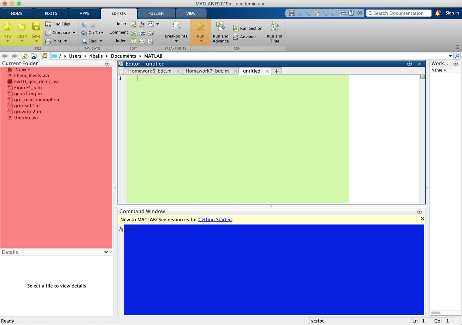
2. We'll call the red pane the File System Viewport. From there we can access a hard drive or network drive and communicate actions we want to perform on the resources that exist there.
3. We'll call the green pane the Script Editor. We can work with MATLAB interactively or through files we edit and run as programs. We will use the word script to refer to programs that run via lines of code that perform many actions at once (because someone else has programmed those services specifically to be run as components in scripts). The script editor is a text editor just like any other text editor you might use for other purposes. But, the script editor is aware it exists within a MATLAB context.
4. We'll call the yellow control the Run Button. The run button lets us execute the current script active in the script editor.
5. We'll call the blue pane the Interactive Command Window. Because MATLAB runs as an interpretive language (one line of code at a time), we can run our code interactively one line at a time (by typing each line of code at the >> prompt and hitting enter or return on the keyboard to see the result of that code cumulatively).
Once you have put the names of interface components above to memory, continue gaining some experience with each:
Let's start with the control that has the most immediacy. We'll create a variable in MATLAB's memory and use a popular function to give it some values. Type:
x = linspace(0,1000,11)into the Interactive Command Window. You should immediately get the response:
x =

  Columns 1 through 8

           0         100         200         300         400         500         600         700

  Columns 9 through 11

         800         900        1000

>>
Your line of code ran a step in a MATLAB script that created a variable named x. That variable now associates eleven numeric values to the label x. Someone else programmed a function and named it linspace. We get used to identifying functions by the use of the parentheses after the function label. Inside of those parenthesis, the programmer let us identify parameters to make the function behave as we wanted it to behave.
In this case we wanted to create a sequence of numbers, equally spaced in value, starting with 0, ending with 1000, and having 11 distinct numbers.
The Interactive Command Window will show you the result of each line of code. Because x is now active as a label in MATLAB's memory, you can type x at any time to see the current values associated with it. And, thanks to MATLAB's unique context, our variable x is also automatically a matrix as well (we'll see how that becomes useful in subsequent primer materials).
Now let's see what happens when MATLAB doesn't understand what we want it to do for us. Type:
x = linespace(0,1000,11)into the Interactive Command Window. You should immediately get the response:
Undefined function or variable 'linespace'.

Did you mean:
>> x = linspace(0,1000,11)
MATLAB feedback usually colors error messages red. The closer we are to entering valid MATLAB syntax, the more useful the error messages will be. The more mistaken we are, the harder the error messages will be to interpret. The goal of this primer is to give you the relevant coding pieces you will need to perform homework in the OCG 351 course. But, you should also use class time to ask questions for clarification when you can't make sense of how to apply the primer to your homework assignments.
We can always use the Interactive Command Window to test out the syntax of lines of code. We can enter a few lines of code in succession to verify a train of thought. But, as our scripts grow in complexity, it is often useful for us to manage our work in files.
Let's create a script file (they normally have a .m extension) from scratch using the Script Editor.
If we click on the New button within the File Controls, we get a sub-menu where the first option is Script. If we click on the Script menu option, a new tab appears in the Script Editor (with a temporary name prefixed by untitled). A text cursor appears in the Script Editor and we can start to type in a new script (as we type an asterisk appears after the tab name — this means the active script in the Script Editor varies from what has been saved — a gentle reminder to save often).
Type two lines of code:
x = linspace(0,1000,11)

x = x + 100
into the Script Editor and click on the Run Button.
We see that MATLAB does not want to run a script from the Script Editor that has not been saved:
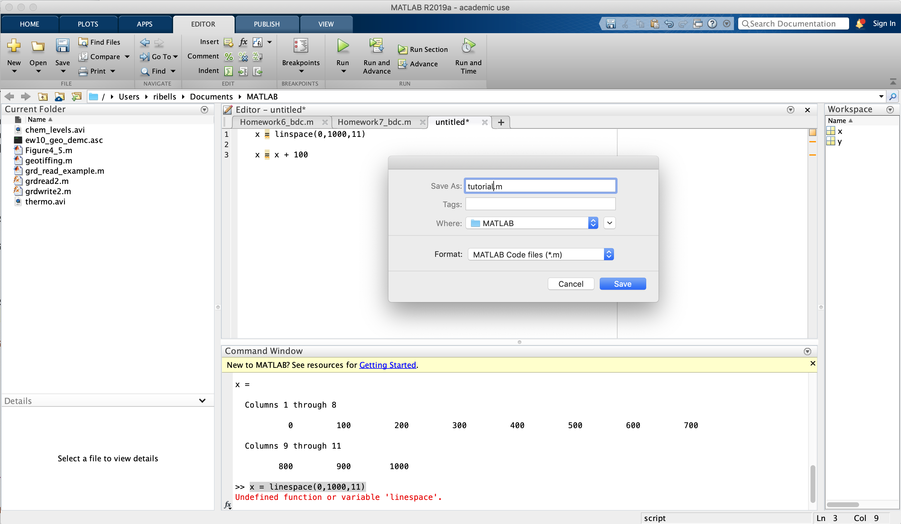
but we can remedy that by naming our script and saving it somewhere within our file system. Let's name it tutorial.m and put it into some folder we know about on our file system (in this case we use the default MATLAB folder that was created by MATLAB when we installed it).
As usual, it makes sense to spend some time thinking about our file system and how we want to organize our scripts for long-term storage and accessibility. If you haven't spent time thinking about file management lately, do get to know your file system, who you share it with, and how best to create a file structure to support this class for you.
When we click Save on the file dialog window, we see there is now a tutorial.m resource listed in the File System Viewport.
We also notice that MATLAB ran the script and put the results of the script into the Interactive Command Window:
>> tutorial

x =

  Columns 1 through 9

           0         100         200         300         400         500         600         700         800

  Columns 10 through 11

         900        1000

x =

  Columns 1 through 9

         100         200         300         400         500         600         700         800         900

  Columns 10 through 11

        1000        1100
Sometimes MATLAB will stop execution of a script when it encounters an error. The error will appear in red within the Interactive Command Window so you can interpret it, make necessary changes to the code, save the script again (using the Save button within the File Controls), and run again (by clicking on the Run Button). This process is often called iterative debugging and is a useful skill to develop with any programming language.
All less significant errors (often called warnings) are worth investigating and cleaning up as well.
We could now build a very comprehensive script within the Script Editor (like the full model analysis shown here). Instead, we will build scripts of increasing complexity within the OCG 351 — with the intent of covering concepts just in time for homework assignments. We can of course gain benefit from doing all the primer modules as soon as you have time and focus to do so. They are all linked here for our convenience:
Primer 1
Primer 2
Primer 3
Primer 4
Primer 5
Primer 6
Primer 7