Now that you've had experience using the MATLAB editor interface and have some experience with matrices, we can continue with specific concepts and skills in subsequent modules. In this module, we'll gain some exposure to 2-D matrix manipulation through for loops. Then, we'll look at a few more useful functions to use when plotting.

Last module we learned about MATLAB's meshgrid function, but then expedited the generation of a 2-D matrix through three lines of code. Let's compress that even tighter to one line of code. Go ahead and create a new MATLAB script (as you did in the basic introduction to the MATLAB editor interface). Let's call it looping.m. Type:

grid = 5+rand(20,30)*10

into the script editor, save the script, and use the Run button to run it. You should see no error messages.

We now have a 2-D matrix (assigned with a label we chose of grid) in MATLAB's managed computing memory.

What properties have we created for this matrix? Well, we know that rand(20,30) creates a 2-D matrix that we can describe as having 20 rows of values and 30 columns of values, with each value being a floating point number between 0 and 1.

The *10 syntax multiplies every value by 10 so that we get values between 0 and 1 (the multiplication runs first according to rules of precedence that dictate every programming language (and MATLAB is conventional here).

The 5+ syntax then adds 5 to each value so that our grid variables contains 600 values between 5 and 15.

Think about what such a grid might represent in terms of a natural phenomenon. Perhaps the grid represents points in a surface of water with values representing temperatures on the Celsius scale. Each time we re-run the grid initialization statement, we get different values for each point in the grid. But, they are all bounded by 5 and 15 each time.

We can write very tight code to perform an operation on each value. Perhaps we are expecting the values to change. We have a simple (and for learning purposes somewhat arbitrary) formula we think will describe how the values will change in the course of the next hour:

temp_new = (25-temp_current)*.01;

In order to get familiar with MATLAB for loops, let's write some code that applies our temperature change formula to each point in our grid matrix, but one value at a time. To access each of the columns of data, we can write a line of code:

for j=1:30

which will initiate a variable named j in memory and then iterate it from 1 to 30 by stepping through the range adding 1 each time.

For the rows of data, we can write a line of code:

for i=1:20

which will initiate a variable named i in memory and then iterate it from 1 to 20 by stepping through the range adding 1 each time.

If we remember that the syntax:

grid(1,1)

represents the value at the intersection of the first row and first column, we can generalize the syntax:

grid(i,j)

to represent the value at the intersection of the j^th row and i^th column.

That syntax is very useful for accessing each grid value within the for loops. We'll update each variable as we access them with code. Add code to your script in the script editor:

for j=1:30
    for i=1:20
        grid(i,j)=grid(i,j)+(25-grid(i,j))*.01
    end
end

and note the indentation of the lines of code to facilitate processing awareness.

And, the indentation does not dictate the behavior of the for loops. It's the for keyword placement in conjunction with the relative end keyword (MATLAB assumes the nesting which is also described as stack behavior) that dictates behavior at runtime.

The first (column-based) loop is outside the second (row-based) loop. Or, said another way, the row-based loop is nested inside the column-based loop.

The order of the loops is irrelevant, but one does need to be nested inside of the other.

When you run the script by clicking on the Run button, you will see MATLAB print out the values of the whole grid each time the grid is updated (600 times) in the Interactive Control Window.

Taking a closer look at the line of code:

grid(i,j)=grid(i,j)+(25-grid(i,j))*.01

we note that the order of precedence is very important in attaining the result we intend to attain.

MATLAB executes the line of code in the following manner:

1. grid(i,j) is read from grid memory and its current value is copied to a computational register.
2. grid(i,j) is read again and its current value is copied to a second computational register.
3. The second register value is updated to subtract its value from 25 (since the subtraction has parentheses around it).
4. The second register value is multiplied by .01.
5. The second register value is added to the first register value.
6. The indexed value in grid memory is updated to hold the same value as the first register.
7. The two registers are released so they can be used in other scratch computation.

Note that other registers are used temporarily to prepare the 25 and .01 values for use but that is of less importance to our understanding of for loops and 2-D matrix computation.

We'll see in a class session how for loops can add additional dimensions to our matrices without much extra work in writing code. For each dimension we add (and as the number of memory locations in those dimensions grow), MATLAB has a lot more work to do to perform the computation we want performed on our behalf.

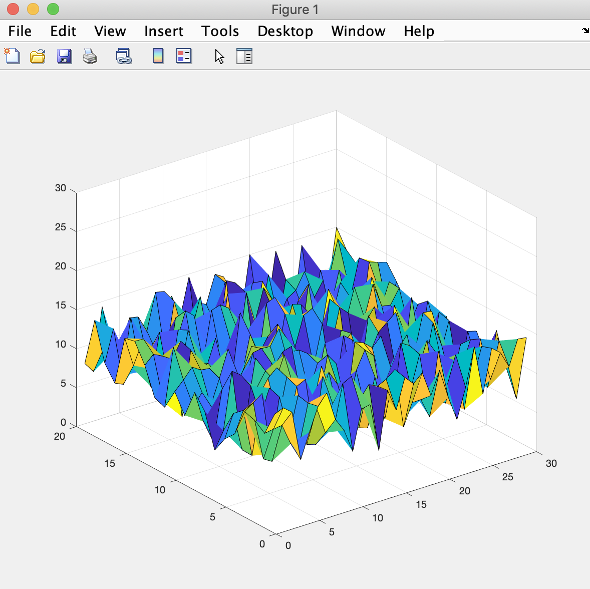
Recall from last module that we can plot the temperature data as a plot using the MATLAB's surf function. Let's add:

surf(grid)
zlim([0 30])

to our script in the Script Editor and then run via the Run button. We get a plot that looks like:



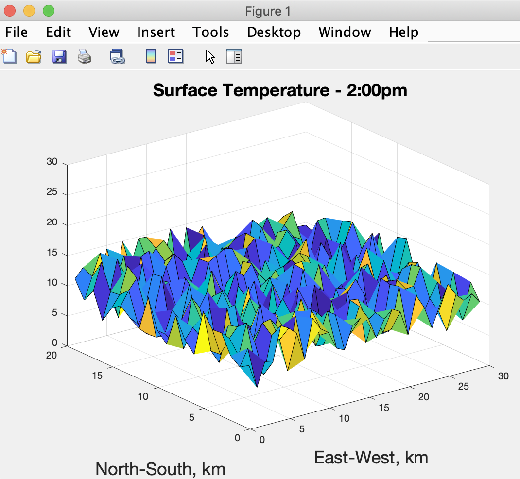
The plot could use some labels to help describe what the plot represents. Add the following three lines to your script in the Script Editor (noting the title, xlabel, and ylabel functions MATLAB provides):

title('\fontsize{18} Surface Temperature - 2:00pm');
ylabel('\fontsize{18} North-South, km');
xlabel('\fontsize{18} East-West, km');

and then run via the Run button. We now get a plot that looks like:



whereby MATLAB has determined the placement of the labels for us.

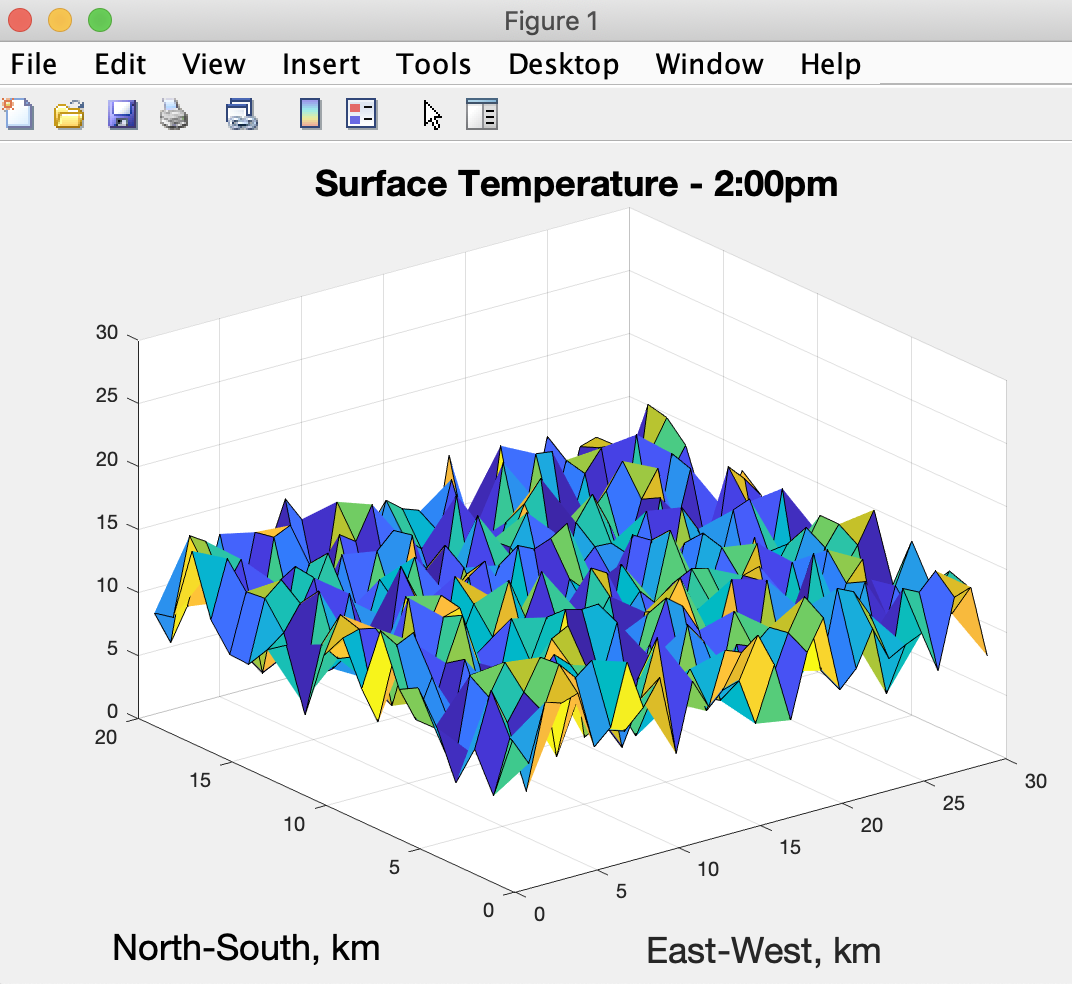
If we don't like the placement of one of the labels, we can always use MATLAB's text function to place it ourselves.

For example, if we don't like where the North-South label appears via the ylabel function, we can replace that line with:

text(-20,4,'North-South, km','fontSize',18)

and then run via the Run button. We now get a plot that looks like:



whereby the North-South label looks more aligned for aethetics (without hurting the communication of its purpose).

There are five parameters to the text function call in this case. The first identifies we want the label to move 20 units to the left. The second identifies we want he label to move 4 units up. The third identifies the text string we want presented, the fourth let's us add the property fontsize, and the fifth sets the fontsize to 18 units.

The MATLAB text reference online describes the units of measure as well as what other optional property declarations we can make with the function.

We can of course gain benefit from continuing with more primer modules or reviewing previous ones. They are all linked here for our convenience:

Introduction
Primer 1
Primer 2
Primer 4
Primer 5
Primer 6
Primer 7