

MATLAB Primer - Module 5
Now that you've had experience using the MATLAB editor interface and have been exposed to a growing sense of matrices, we can continue with specific concepts and skills in subsequent modules. In this module, we'll continue our exposure to plotting with the plot function while also investigating subroutines. This module builds significantly upon the previous module, module 4.
We will start off by initializing a 2-D matrix with a different number of rows and columns than we used last module.
Let's see if we can anticipate the shape of a 2-D matrix as we start a new script in the MATLAB editor interface. Create
a new script and call it matrix3.m. Then start the script off by copying:
We now have a 2-D matrix (assigned with a label we chose of T) in MATLAB's managed computing memory.
What is the shape of matrix T in memory?
To review, we note that each row in memory ends with a semi-colon when using the syntax we've used here to initialize matrix T. The last row does not need to end in a semi-colon because the closing square-bracket ends the structure declaration.
With the arbitrary use of end-of-line characters (which are unprintable), there are three rows initialized per line of code. And with six lines of code, there are 18 rows declared in total.
Each of those rows has four values in it (delimited by space characters). So matrix T has 18 rows and 4 columns.
We can test our understanding by requesting MATLAB to print out the value in the 15th row and third column.
If we add a line of code:
That value is the same value as the matrix element colored green above, verifying our expectation.
Remember that in the last module we considered the 2-D matrix T to contain temperature values that changed over time in a simulation. Let's do the same here and track twelve temperatures (at 4 longitudes and 3 latitudes) over six time steps. Consider that the simulation has already been run and matrix T contains the final results of our simulation.
Remember also that in the last module we introduced six lines of code that would repackage a 2-D matrix of results into a useful 3-D package of results. We'll do the same here, but we'll investigate subroutines while we do so.
MATLAB programming makes use of subroutines to reuse useful groups of code statements across projects. Programmers learn a skill to write subroutines at the best level of generality for reuse, but we'll just start with a naive subroutine that is specific to the structure of our 2-D matrix T.
Unlike other programming languages, MATLAB prefers that we specify subroutines at the bottom of a script file (and at run-time MATLAB always searches all the way to the bottom of a file to find them).
Let's add the following subroutine to the bottom of our script file in the Script Editor:
We've added a first line to package those lines as a subroutine. MATLAB expects us to be declaring a subroutine when it encounters the function keyword. It then evaluates the rest of a line that starts with the keyword function as follows:
1. The label that appears within the square-brackets just right of the word function is evaluated as a variable that will be returned to the calling script (in this case a three_d matrix),
2. an equal sign follows the return declaration and then a name for the subroutine appears before the parentheses, and
3. any parameters to be passed into the subroutine appear within the parentheses.
The square brackets and parentheses can be empty. So the line of code would be valid as:
function [] = package()
but in that case the subroutine would not likely be very flexible.
More typically, the square brackets and parentheses contain multiple variables. So the line of code would also be valid as: function [three_d, depth] = package(two_d, column_size)
and we could then write a more general subroutine that handled varying sizes of rows.
We can find many tutorials and reference pages for more information on creating local functions. Suffice to say here, the skill is a nuanced skill developed with study and practice in a computer science curriculum.
We can now call our subroutine from within our script.
Let's add a line of code to call our subroutine. Type:
MATLAB runs our calling line of code as follows:
1. MATLAB finds the function declaration associated with our label package, 2. It notes that the signature of the function requires a single parameter and passes our matrix T into the function as the one parameter required, 3. MATLAB runs the subroutine, using our matrix T in the variable two_d specified in the subroutine, 4. MATLAB initializes a variable with a temporary label of three_d in which it builds a 3-D matrix, 5. MATLAB returns the contents of the three_d variable's memory to be initialized as a matrix Tsim, and 6. MATLAB releases the memory used by the subroutine (those locations labeled as two_d and three_d).
As a result of the subroutine we are left with a 3-D matrix named Tsim, which is very similar in purpose to the Tsim we used in the last module.
To test that the subroutine worked properly, we can type:
None of this should be a surprise if we mastered the previous module. We've just cleaned up our coding approach a bit to identify a verbose process for use by a single line of code.
If we think about that for a bit, we realize all the functions we have used in this MATLAB primer have to have been declared somewhere after being written by some programmer or programmers. We've now looked inside a bit by writing our own function. And, perhaps, we can anticipate that it is a good idea not to use a label for our subroutines that are already used by MATLAB.
When we do a Google search upon the phrase matlab package function we find the search results include information about packages and how to package code, but without mention of any built-in function called package.
Still, it would probably be a good idea to create a better label like packageTwoDMatrixAsThreeD that would be unlikely to clash with built-in function names for future releases of MATLAB.
Note we'd then have to change two labels in our code: the label used to declare the function, and the label used to call the function.
Let's now return to plotting our simulation results. In the last module, we used the surf function to specifically request a surface plot of our data.
MATLAB contains flexible plot and pcolor functions.
The MATLAB plot function lets us plot points in 2-D efficiently. It is very powerful in its ability to create a plot from implicit expectation of our intent. Usually, the plot function expects two parameters as explicit x and y values (which then must be of the same size). For example:
which draws line segments from each set of coordinates using the indices into matrices x and y.
But looks what happens if we request:
which is a plot of temperature values for our four column (longitude) values over the 18 rows we have in memory.
As a result, the plot shows the general increase in temperature for all points in our T matrix, with some default colors that MATLAB choses for readability.
But, if we request:
Let's add the following lines of code to our script, just above the subroutine we have at the bottom:
Run the script by clicking on the Run button and MATLAB should create six figures that look like:
whereby each figure shows the temperatures plotted for a time step (longitude varying horizontally and latitude varying vertically).
Looking at the figures in succession provides a sense of how the temperature spread changes over time, but does not suggest an increasing temperature trend (we'll add additional code next module to help with that). The change in relative spread is nuanced but visible.
In the code, we see that the pcolor function takes a sequence of data out of the 3-D matrix Tsim as a parameter.
The sequence requests all rows and all columns for a specific page of matrix Tsim (and each page is indexed by a time step index from 1 to 6).
The code suggests the use of a linear interpolation between data points (as we saw the plot function did for 2-D data).
And the code explicitly requests the use of the jet colormap. The jet colormap is a rainbow-based colormap that scientists have made popular through use over many years. There are many other colormap options we can use via the appropriate keyword.
We will continue plotting with the pcolor function next module.
We can of course gain benefit from continuing with more primer modules or reviewing previous ones. They are all linked here for our convenience:
Introduction
Primer 1
Primer 2
Primer 3
Primer 4
Primer 6
Primer 7
T = [14.9 15.0 15.2 15.4; 14.2 14.3 14.5 14.7; 13.4 13.69 13.9 14.2;
15.001 15.1 15.298 15.4; 14.308 14.407 14.605 14.7; 13.5160 13.8031 14.0110 14.2;
15.101 15.199 15.395 15.591; 14.4149 14.5129 14.7089 14.905; 13.6308 13.9151 14.1209 14.4149;
15.2 15.297 15.4911 15.6851; 14.5208 14.6178 14.8119 15.0059; 13.7445 14.0259 14.2297 14.4149;
15.298 15.394 15.5862 15.7783; 14.6256 14.7216 14.9137 15.1059; 13.8571 14.1357 14.3374 14.6256;
15.395 15.4901 15.6803 15.8705; 14.7293 14.8244 15.0146 15.2048; 13.9685 14.2443 14.4440 14.7293]
and pasting it into the Script Editor. Save the script, and use the Run button to run it. You should see no error messages.
We now have a 2-D matrix (assigned with a label we chose of T) in MATLAB's managed computing memory.
What is the shape of matrix T in memory?
To review, we note that each row in memory ends with a semi-colon when using the syntax we've used here to initialize matrix T. The last row does not need to end in a semi-colon because the closing square-bracket ends the structure declaration.
With the arbitrary use of end-of-line characters (which are unprintable), there are three rows initialized per line of code. And with six lines of code, there are 18 rows declared in total.
Each of those rows has four values in it (delimited by space characters). So matrix T has 18 rows and 4 columns.
We can test our understanding by requesting MATLAB to print out the value in the 15th row and third column.
If we add a line of code:
T(15,3)we see the value 14.3374 print out as an answer in the Interactive Control Window.
That value is the same value as the matrix element colored green above, verifying our expectation.
Remember that in the last module we considered the 2-D matrix T to contain temperature values that changed over time in a simulation. Let's do the same here and track twelve temperatures (at 4 longitudes and 3 latitudes) over six time steps. Consider that the simulation has already been run and matrix T contains the final results of our simulation.
Remember also that in the last module we introduced six lines of code that would repackage a 2-D matrix of results into a useful 3-D package of results. We'll do the same here, but we'll investigate subroutines while we do so.
MATLAB programming makes use of subroutines to reuse useful groups of code statements across projects. Programmers learn a skill to write subroutines at the best level of generality for reuse, but we'll just start with a naive subroutine that is specific to the structure of our 2-D matrix T.
Unlike other programming languages, MATLAB prefers that we specify subroutines at the bottom of a script file (and at run-time MATLAB always searches all the way to the bottom of a file to find them).
Let's add the following subroutine to the bottom of our script file in the Script Editor:
function [three_d] = package(two_d)
    three_d = two_d(1:3,:)
    three_d = cat(3,three_d,[two_d(4:6,:)])
    three_d = cat(3,three_d,[two_d(7:9,:)])
    three_d = cat(3,three_d,[two_d(10:12,:)])
    three_d = cat(3,three_d,[two_d(13:15,:)])
    three_d = cat(3,three_d,[two_d(16:18,:)])
end
The middle six lines of code should look familiar as similar to the code we used in the last module.
We've added a first line to package those lines as a subroutine. MATLAB expects us to be declaring a subroutine when it encounters the function keyword. It then evaluates the rest of a line that starts with the keyword function as follows:
1. The label that appears within the square-brackets just right of the word function is evaluated as a variable that will be returned to the calling script (in this case a three_d matrix),
2. an equal sign follows the return declaration and then a name for the subroutine appears before the parentheses, and
3. any parameters to be passed into the subroutine appear within the parentheses.
The square brackets and parentheses can be empty. So the line of code would be valid as:
function [] = package()
but in that case the subroutine would not likely be very flexible.
More typically, the square brackets and parentheses contain multiple variables. So the line of code would also be valid as: function [three_d, depth] = package(two_d, column_size)
and we could then write a more general subroutine that handled varying sizes of rows.
We can find many tutorials and reference pages for more information on creating local functions. Suffice to say here, the skill is a nuanced skill developed with study and practice in a computer science curriculum.
We can now call our subroutine from within our script.
Let's add a line of code to call our subroutine. Type:
Tsim = package(T)below our matrix T initialization and above our subroutine.
MATLAB runs our calling line of code as follows:
1. MATLAB finds the function declaration associated with our label package, 2. It notes that the signature of the function requires a single parameter and passes our matrix T into the function as the one parameter required, 3. MATLAB runs the subroutine, using our matrix T in the variable two_d specified in the subroutine, 4. MATLAB initializes a variable with a temporary label of three_d in which it builds a 3-D matrix, 5. MATLAB returns the contents of the three_d variable's memory to be initialized as a matrix Tsim, and 6. MATLAB releases the memory used by the subroutine (those locations labeled as two_d and three_d).
As a result of the subroutine we are left with a 3-D matrix named Tsim, which is very similar in purpose to the Tsim we used in the last module.
To test that the subroutine worked properly, we can type:
Tsim(3,3,5)into the Interactive Control Window, and see the answer of:
ans =

14.3374
appear in response. That's the same value we requested as T(15,3) where T is a 2-D matrix collection of the same values.
None of this should be a surprise if we mastered the previous module. We've just cleaned up our coding approach a bit to identify a verbose process for use by a single line of code.
If we think about that for a bit, we realize all the functions we have used in this MATLAB primer have to have been declared somewhere after being written by some programmer or programmers. We've now looked inside a bit by writing our own function. And, perhaps, we can anticipate that it is a good idea not to use a label for our subroutines that are already used by MATLAB.
When we do a Google search upon the phrase matlab package function we find the search results include information about packages and how to package code, but without mention of any built-in function called package.
Still, it would probably be a good idea to create a better label like packageTwoDMatrixAsThreeD that would be unlikely to clash with built-in function names for future releases of MATLAB.
Note we'd then have to change two labels in our code: the label used to declare the function, and the label used to call the function.
Let's now return to plotting our simulation results. In the last module, we used the surf function to specifically request a surface plot of our data.
MATLAB contains flexible plot and pcolor functions.
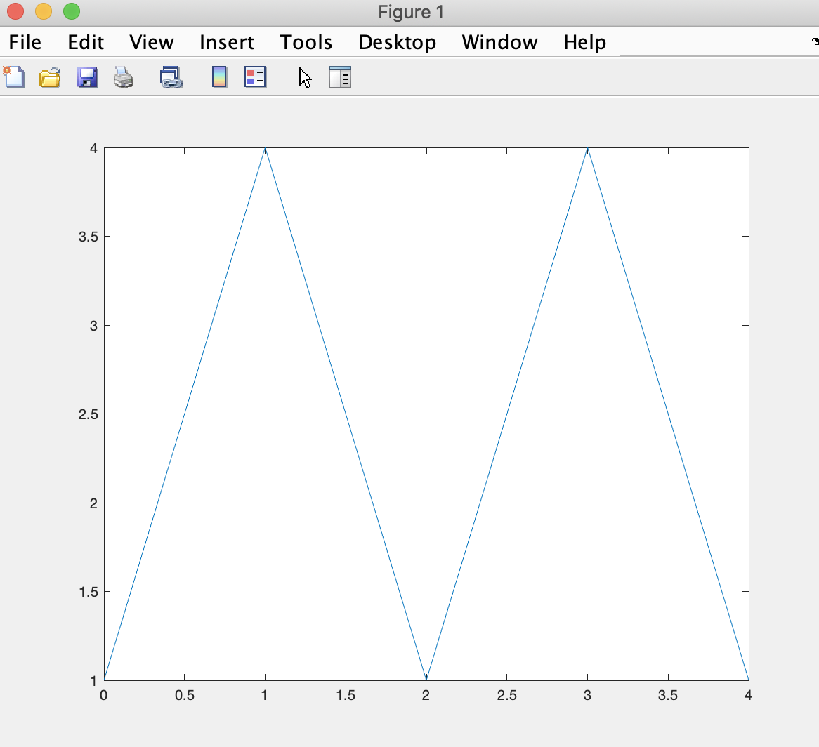
The MATLAB plot function lets us plot points in 2-D efficiently. It is very powerful in its ability to create a plot from implicit expectation of our intent. Usually, the plot function expects two parameters as explicit x and y values (which then must be of the same size). For example:
x=[0 1 2 3 4]
y=[1 4 1 4 1]
plot(x,y)
creates the plot:
which draws line segments from each set of coordinates using the indices into matrices x and y.
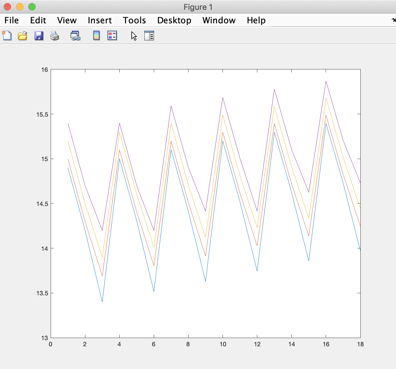
But looks what happens if we request:
plot(T)MATLAB creates the plot:
which is a plot of temperature values for our four column (longitude) values over the 18 rows we have in memory.
As a result, the plot shows the general increase in temperature for all points in our T matrix, with some default colors that MATLAB choses for readability.
But, if we request:
plot(Tsim)MATLAB responds with an error message in the Interactive Control Window:
Error using plot
Data cannot have more than 2 dimensions.
It turns out that the pcolor function is particularly useful for showing 3-D data whereby one of the dimensions is time.
Let's add the following lines of code to our script, just above the subroutine we have at the bottom:
for time=1:6
    figure
    pcolor(Tsim(:,:,time))
    shading interp
    colormap jet
end
so that our code is complete as:
T = [14.9 15.0 15.2 15.4; 14.2 14.3 14.5 14.7; 13.4 13.69 13.9 14.2;
15.001 15.1 15.298 15.4; 14.308 14.407 14.605 14.7; 13.5160 13.8031 14.0110 14.2;
15.101 15.199 15.395 15.591; 14.4149 14.5129 14.7089 14.905; 13.6308 13.9151 14.1209 14.4149;
15.2 15.297 15.4911 15.6851; 14.5208 14.6178 14.8119 15.0059; 13.7445 14.0259 14.2297 14.4149;
15.298 15.394 15.5862 15.7783; 14.6256 14.7216 14.9137 15.1059; 13.8571 14.1357 14.3374 14.6256;
15.395 15.4901 15.6803 15.8705; 14.7293 14.8244 15.0146 15.2048; 13.9685 14.2443 14.4440 14.7293]

Tsim = package(T)

for time=1:6
    figure
    pcolor(Tsim(:,:,time))
    shading interp
    colormap jet
end

function [three_d] = package(two_d)
    three_d = two_d(1:3,:)
    three_d = cat(3,three_d,[two_d(4:6,:)])
    three_d = cat(3,three_d,[two_d(7:9,:)])
    three_d = cat(3,three_d,[two_d(10:12,:)])
    three_d = cat(3,three_d,[two_d(13:15,:)])
    three_d = cat(3,three_d,[two_d(16:18,:)])
end
in the Script Editor.
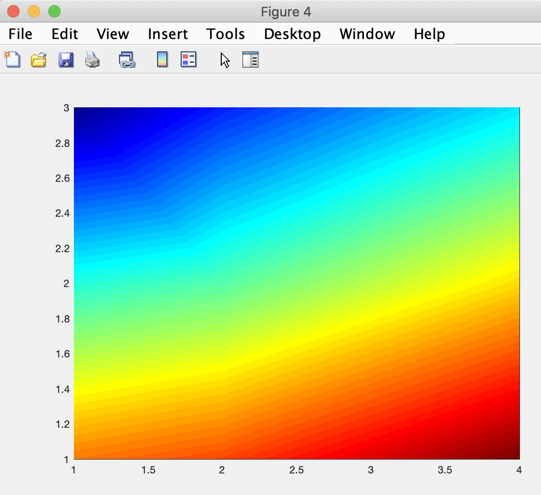
Run the script by clicking on the Run button and MATLAB should create six figures that look like:
whereby each figure shows the temperatures plotted for a time step (longitude varying horizontally and latitude varying vertically).
Looking at the figures in succession provides a sense of how the temperature spread changes over time, but does not suggest an increasing temperature trend (we'll add additional code next module to help with that). The change in relative spread is nuanced but visible.
In the code, we see that the pcolor function takes a sequence of data out of the 3-D matrix Tsim as a parameter.
The sequence requests all rows and all columns for a specific page of matrix Tsim (and each page is indexed by a time step index from 1 to 6).
The code suggests the use of a linear interpolation between data points (as we saw the plot function did for 2-D data).
And the code explicitly requests the use of the jet colormap. The jet colormap is a rainbow-based colormap that scientists have made popular through use over many years. There are many other colormap options we can use via the appropriate keyword.
We will continue plotting with the pcolor function next module.
We can of course gain benefit from continuing with more primer modules or reviewing previous ones. They are all linked here for our convenience:
Introduction
Primer 1
Primer 2
Primer 3
Primer 4
Primer 6
Primer 7