Now that you've had experience using the MATLAB editor interface and have been exposed to a growing sense of matrices, we can continue with specific concepts and skills in subsequent modules. In this module, we'll continue our exposure to 2-D matrices — focusing on their shape and significance of that shape. Then, we'll continue looking useful keywords to use when plotting.

To follow along with a more complex 2-D matrix example, let's create a new MATLAB script (as you did in the basic introduction to the MATLAB editor interface) and call it matrix2.m. Start off by copying:

T=[24.9 25.0 25.2 25.4 25.6 25.8 26.0 26.2 26.5 26.8 27.0 27.3 27.5 28;
    22.2 22.3 22.5 22.7 22.9 23.1 23.35 23.55 23.8 24 24.4 24.8 25.2 26;
    21.6 21.8 22.1 22.25 22.4 22.6 22.75 22.95 23.15 23.4 23.69 23.9 24.2 24.8;
    21.1 21.3 21.5 21.7 21.9 22.05 22.25 22.42 22.62 22.81 23.01 23.2 23.45 23.68;
    20.6 20.8 20.95 21.15 21.39 21.59 21.75 21.9 22.15 22.38 22.55 22.75 22.9 23.15;
    20.15 20.29 20.48 20.68 20.9 21.05 21.2 21.4 21.6 21.85 22.05 22.25 22.48 22.69;
    19.2 19.6 19.9 20.15 20.35 20.55 20.7 20.9 21.1 21.28 21.5 21.7 21.95 22.2;
    18.2 18.6 19.1 19.45 19.8 20.05 20.25 20.44 20.65 20.85 21.05 21.2 21.4 21.65;
    16.7 17.1 17.6 17.9 18.25 18.50 18.8 19.00 19.25 19.4 19.7 19.9 20.1 20.2]

and pasting it into the Script Editor. Save the script, and use the Run button to run it. You should see no error messages.

We now have a 2-D matrix (assigned with a label we chose of T) in MATLAB's managed computing memory.

Let's consider matrix T to be a snapshot of temperature values (Celsius) for a body of water where there is a uniform distance between temperature locations within each row. We have locations in fourteen columns reflecting longitudes east to west, and we have nine rows reflecting nine different latitudes from north to south.

If we add a line of code:

T(5,6)

we see the value 21.5900 print out as an answer in the Interactive Control Window.

That value is the same value as the matrix element colored green above. It exists as the value at the intersection of the fifth row with the sixth column.

To adopt the code we worked with in the last module (module 3) to work with this 2-D matrix, we add:

for j=1:14
    for i=1:9
        T(i,j)=T(i,j)+(25-T(i,j))*.01
    end
end

to our script in the Script Editor.

Those five lines of code update each temperature value with the next value in a somewhat arbitrary (contrived) warming scenario simulation.

We can nest those lines inside of a time-stepping loop (with two new lines of code):

for time = 1:5
	for j=1:14
		for i=1:9
			T(i,j)=T(i,j)+(25-T(i,j))*.01
		end
	end
end

whereby a variable we name time keeps track of five timesteps (we can consider them to be hourly).

The code should run without any errors appearing in the Interactive Control Window.

At that point, our matrix T contains simulated values for temperatures five time steps (hours) after the data initialized in matrix T were recorded.

But note that this approach throws away intermediary values for temperature in matrix T as the next time step's computation is performed.

Often a modeler will want to keep intermediary values in order to use them in an analysis after a simulation has run.

We can do that by appending to matrix T for each time step (or by creating a much larger T to hold those values at matrix initialization).

Since this module is about the flexibility of matrices, we'll grow matrix T as we compute. We know we need 9x14 new values in the matrix for each timestep. One simple method is to use a temporary matrix we can concatenate to a growing matrix T. In that case:

1. we create a start_row variable to keep track of the start of a timestep's row location,
2. we capture the result of each temperature update function in a temporary matrix (named temp below) while moving through our expanding matrix T,
3. we use the vertcat function to expand matrix T to append the new timestep values held in matrix temp, and
4. we update the start_row variable to move nine rows further down for the next timestep.

start_row = 0
for time = 1:5
	for j=1:14
		for i=1:9
			temp(i,j)=T(start_row+i,j)+(25-T(start_row+i,j))*.01
		end
    end
    T = vertcat(T,temp)
    start_row = start_row + 9
end

When we are done running the script, matrix T still has fourteen columns, but now has 54 rows for the nine latitudes we are interested in across six different times (our initial time, as well as five additional ones created as timesteps in a simulation.

MATLAB has some very clever syntax for working with arrays and we can move our 2-D matrix into a 3-D matrix by treating time as another dimension.

Consider this line of code:

T(1:9,:)

which asks for a subset of data from matrix T.

This syntax requests for the sequence of rows 1 through 9 for all columns, which is exactly the data we started with.

With that train of thought, we see that:

T(10:18,:)

represents the data for a subset of matrix T that holds just the values for the timestep 1 hour after the initial data (rows 10 through 18 with all columns requested).

Our last timestep's data is represented by:

T(46:54,:)

MATLAB's memory manipulations include the ability to create a 3-D matrix from any 2-D matrix that encodes a pattern for the extra dimension.

We can create the 3-D matrix we want by concatenating the six time steps together into a 3-D matrix (the first parameter of 3 in the cat function):

Tsim = [T(1:9,:)]
Tsim = cat(3,Tsim,[T(10:18,:)])
Tsim = cat(3,Tsim,[T(19:27,:)])
Tsim = cat(3,Tsim,[T(28:36,:)])
Tsim = cat(3,Tsim,[T(37:45,:)])
Tsim = cat(3,Tsim,[T(46:54,:)])

The 3-D format is nice because we can then refer to any particular value through three indices. For example:

Tsim(7,2,4)

represents the value at latitude 7, longitude 2, and timestep 4 (which is the third timestep from our loop, the initial data is indexed as 1). The Interactive Control Window responds to that line of code with:

ans =

   19.6540

without any errors.

To gain a deeper understanding (and reinforce what we've done so far), we can review the multidimensional array documentation from the MATLAB online reference.

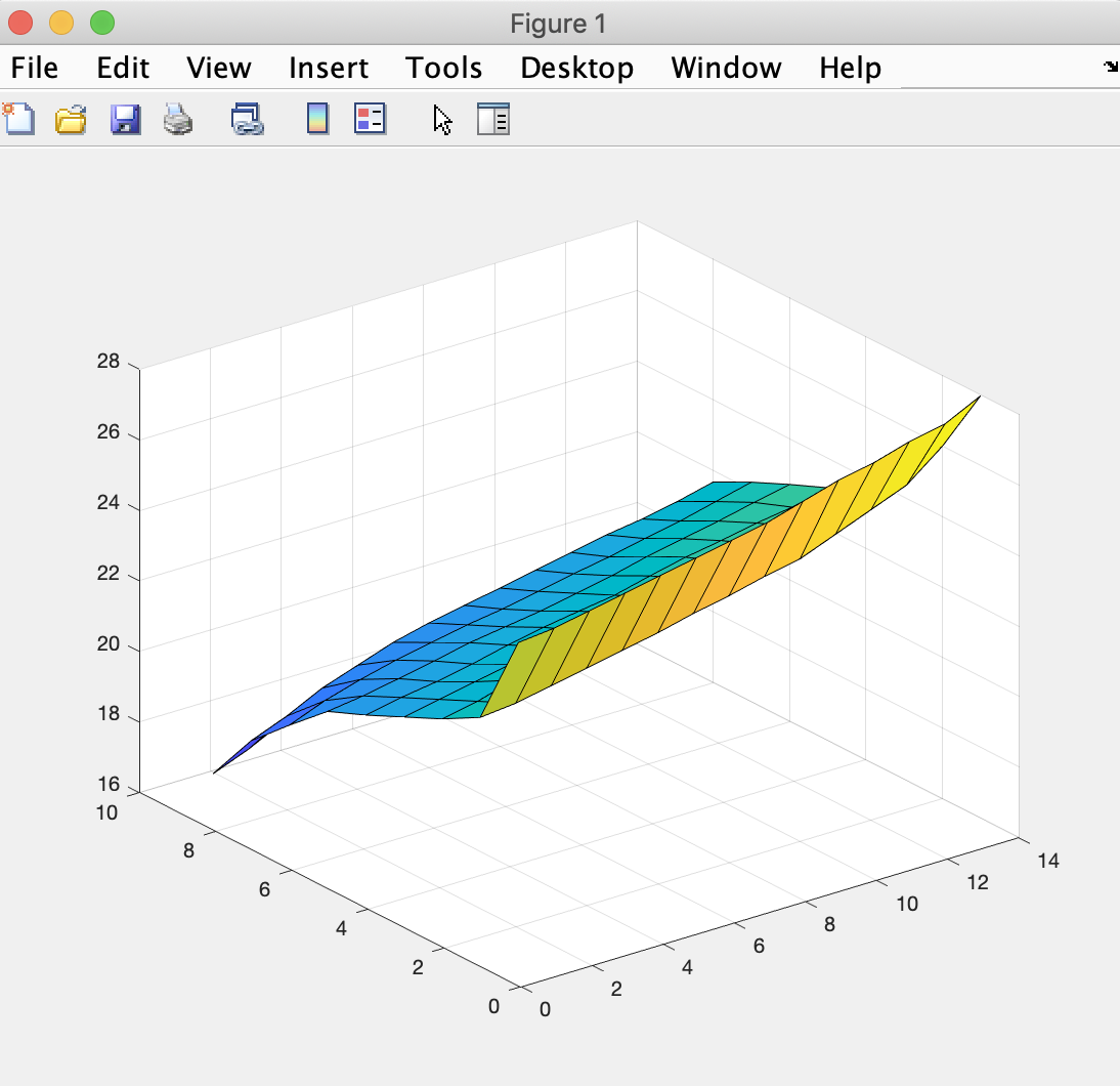
At this point, we can use the surf function to see a surface representation of temperatures for any timestep. Note that:

surf(T(19:27,:))

and

surf(Tsim(:,:,3)

are an identical request for a plot that looks like:



with the difference being how the data is being stored (in an appended 2-D array or 3-D array).

Let's put it all together in a script that shows plots for all six timesteps (our initial and five additional):

T=[24.9 25.0 25.2 25.4 25.6 25.8 26.0 26.2 26.5 26.8 27.0 27.3 27.5 28;
    22.2 22.3 22.5 22.7 22.9 23.1 23.35 23.55 23.8 24 24.4 24.8 25.2 26;
    21.6 21.8 22.1 22.25 22.4 22.6 22.75 22.95 23.15 23.4 23.69 23.9 24.2 24.8;
    21.1 21.3 21.5 21.7 21.9 22.05 22.25 22.42 22.62 22.81 23.01 23.2 23.45 23.68;
    20.6 20.8 20.95 21.15 21.39 21.59 21.75 21.9 22.15 22.38 22.55 22.75 22.9 23.15;
    20.15 20.29 20.48 20.68 20.9 21.05 21.2 21.4 21.6 21.85 22.05 22.25 22.48 22.69;
    19.2 19.6 19.9 20.15 20.35 20.55 20.7 20.9 21.1 21.28 21.5 21.7 21.95 22.2;
    18.2 18.6 19.1 19.45 19.8 20.05 20.25 20.44 20.65 20.85 21.05 21.2 21.4 21.65;
    16.7 17.1 17.6 17.9 18.25 18.50 18.8 19.00 19.25 19.4 19.7 19.9 20.1 20.2]

start_row = 0;

%run the simulation for five more timesteps
for time = 1:5
	for j=1:14
		for i=1:9
			temp(i,j)=T(i+start_row,j)+(25-T(i+start_row,j))*.01
		end
    end
    T = vertcat(T,temp)
    start_row = start_row + 9
    figure
    surf(T(start_row+1:start_row+9,:))
end

MATLAB provides the keyword figure we can use to create multiple plots from within the same script (as used near the bottom of the script above).

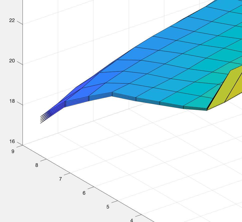
Comparing figure 1 with figure 6, we notice that the plots show that the temperatures move very little over five hours.



To verify that visual conclusion, we can create a single figure that contains six surfaces. To do that change the end of the script from:

    surf(T(start_row+1:start_row+9,:))
end

to add two lines strategically:

    surf(T(start_row+1:start_row+9,:))
    hold on
end
hold off

and then we can see the layering of six surfaces in the lower-left corner of the surfaces:



Lastly, we create a version using a pre-defined 3-D matrix we fill with the simulation. This makes sense when we know in advance how many timesteps we want to run our simulation for:

T = zeros(9,14,6)

T(:,:,1) =[24.9 25.0 25.2 25.4 25.6 25.8 26.0 26.2 26.5 26.8 27.0 27.3 27.5 28;
    22.2 22.3 22.5 22.7 22.9 23.1 23.35 23.55 23.8 24 24.4 24.8 25.2 26;
    21.6 21.8 22.1 22.25 22.4 22.6 22.75 22.95 23.15 23.4 23.69 23.9 24.2 24.8;
    21.1 21.3 21.5 21.7 21.9 22.05 22.25 22.42 22.62 22.81 23.01 23.2 23.45 23.68;
    20.6 20.8 20.95 21.15 21.39 21.59 21.75 21.9 22.15 22.38 22.55 22.75 22.9 23.15;
    20.15 20.29 20.48 20.68 20.9 21.05 21.2 21.4 21.6 21.85 22.05 22.25 22.48 22.69;
    19.2 19.6 19.9 20.15 20.35 20.55 20.7 20.9 21.1 21.28 21.5 21.7 21.95 22.2;
    18.2 18.6 19.1 19.45 19.8 20.05 20.25 20.44 20.65 20.85 21.05 21.2 21.4 21.65;
    16.7 17.1 17.6 17.9 18.25 18.50 18.8 19.00 19.25 19.4 19.7 19.9 20.1 20.2]

surf(T(:,:,1))
hold on

%run the simulation for five more timesteps
for time=1:5
	for j=1:14
		for i=1:9
			T(i,j,time+1)=T(i,j,time)+(25-T(i,j,time))*.01
		end
    end
    surf(T(:,:,time+1))
    hold on
end

hold off

The first line sets up a 3-D matrix in MATLAB memory that has room for 9 rows, 14 columns, and 6 pages (if we think of each timestep of rows and columns a page).

The second line fills the first page with initialization values and then our timestep loop creates and stores five additional pages (one per timestep).

Our surf function accesses one page at a time to add to the figure we are plotting. And the resulting figure is identical to the image above.

We can of course gain benefit from continuing with more primer modules or reviewing previous ones. They are all linked here for our convenience:

Introduction
Primer 1
Primer 2
Primer 3
Primer 5
Primer 6
Primer 7