Now that you've had experience using the MATLAB editor interface and have been exposed to a growing sense of matrices, we can continue with specific concepts and skills in subsequent modules. In this module, we'll continue our exposure to plotting with the plot function, focusing on how to extract desired data from a 3-D matrix.

We will start off by initializing a 3-D matrix with the data we used last module. Let's see if we can anticipate the shape of a 3-D matrix as we start a new script in the MATLAB editor interface. Create a new script and call it matrix4.m. Then start the script off by copying:

T = [14.9 15.0 15.2 15.4; 14.2 14.3 14.5 14.7; 13.4 13.69 13.9 14.2]
T(:,:,2) = [15.001 15.14 15.298 15.4; 14.38 14.407 14.65 14.7; 13.516 13.8031 14.0110 14.2]
T(:,:,3) = [15.121 15.3 15.39 15.91; 14.449 14.129 14.789 14.95; 13.638 13.51 14.209 14.449]
T(:,:,4) = [15.32 15.297 15.11 15.51; 14.208 14.178 14.119 15.57; 13.745 14.259 14.297 14.149]
T(:,:,5) = [15.28 15.22 15.582 15.783; 14.656 14.216 14.37 15.59; 13.571 14.357 14.374 14.256]
T(:,:,6) = [15.395 15.401 15.803 15.805; 14.793 14.244 15.46 15.20; 13.685 14.443 14.444 14.793]

and pasting it into the Script Editor. Save the script, and use the Run button to run it. You should see no error messages.

We now have a 3-D matrix (assigned with a label we chose of T) in MATLAB's managed computing memory.

The 3-D matrix T is similar to the 3-D matrix Tsim we saw last module, except the data represents actual data, not the simulation following a simple linear change formula.

We initialize matrix T one page at a time (each line of code is a page representing a later timestep).

Now we can use matrix T to plot out some perspectives on the data.

Let's add a time vector to our script (with values for the number of hours since start at each timestep):

time = [0,1,2,3,4,5]

We can extract the change over time for the southwest most location from matrix T using MATLAB's squeeze function:

squeeze(T(1,1,:))

which returns a 1-D vector. Since we have six timesteps and six time elements (in hours), we can use the plot function to plot the temperature at that location over time:

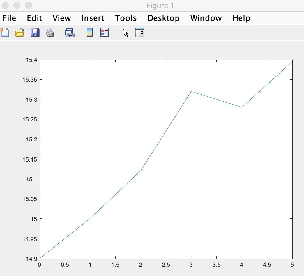
plot(time, squeeze(T(1,1,:)))

MATLAB creates a plot figure:



which shows the temperature changing from 14.9 to 15.4 degrees in five hours.

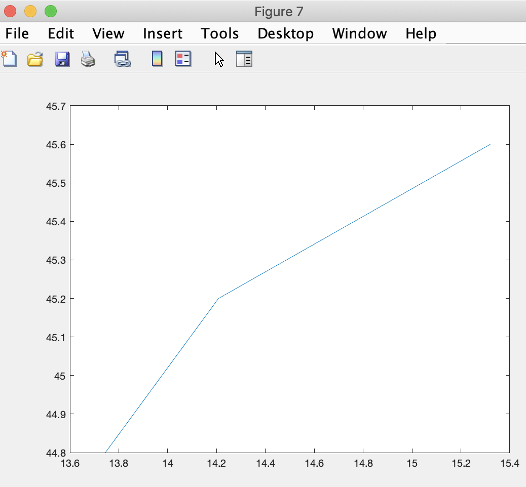
The squeeze function can pull out a sequence of values in any of the three dimensions. So, we can alternatively plot the temperatures for one longitude at a timestep with the line of code (the west most longitude for all latitudes):

plot(squeeze(T(:,1,4)), [45.6,45.2,44.8])

that requests the plot figure:



where it makes sense to show latitude on the horizontal axis.

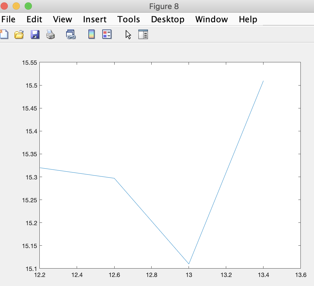
To plot the values along one latitude, we squeeze as follows in a line of code:

plot([12.2,12.6,13.0,13.4], squeeze(T(1,:,4)))

that generates the plot: MATLAB creates the plot figure:



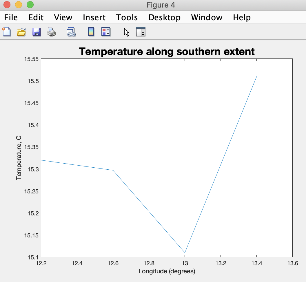
Of course we can add labels to each plot with added code:

xlabel('Longitude (degrees)')
ylabel('Temperature, C')
text(140,32,'Time is 3 hours')
title('Temperature along southern extent','FontSize', 18)

to make them more immediately interpretable:



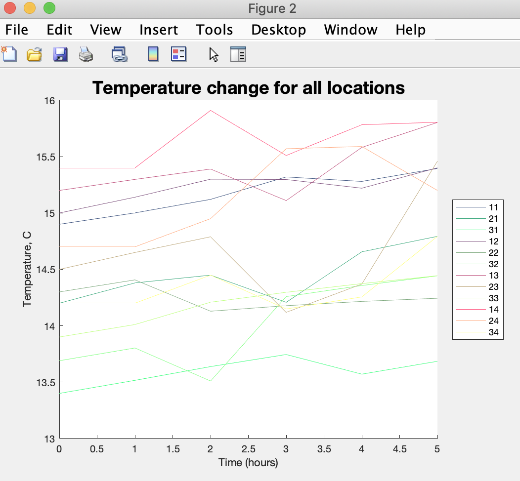
Let's plot the change in temperature for all twelve locations we're monitoring on one figure.

We can do so by adding this code to the bottom of our script in the Script Editor:

figure
hold on
for j=1:4
    for i=1:3
        plot(time, squeeze(T(i,j,:)),'DisplayName',strcat(int2str(i),int2str(j)),'Color',[j/4 i/3 .5])
    end
end
hold off
xlabel('Time (hours)')
ylabel('Temperature, C')
title('Temperature change for all locations','FontSize', 18)
lgd = legend('Location', 'eastoutside')
lgd.NumColumns = 1

which generates the figure:



that has an added legend to the figure and used a red, green, blue specification of color for each line (using the [R G B] notation where each element is between 0 (no intensity) and 1 (full intensity).

We can of course gain benefit from continuing with one more primer module or reviewing previous ones. They are all linked here for our convenience:

Introduction
Primer 1
Primer 2
Primer 3
Primer 4
Primer 5
Primer 7