

MATLAB Primer - Module 2
Now that you've had a basic introduction to the MATLAB editor interface and have a basic sense of matrices, we can continue with specific concepts and skills in subsequent modules. In this module, we'll gain exposure to sequences, 2-D matrices, meshgrids, and continue our thoughts on plotting.
We started learning about MATLAB via the linspace function. MATLAB provides
a simple colon operator for making a sequence of integers that vary by 1 between elements. If we type:
whereby MATLAB considers variable x a matrix (and in this case also a vector as it is a one-dimensional matrix) that contains five
values from 1 to 5. We can then access the matrix to make changes to the values via the indexing syntax we reviewed in
the last tutorial module.
For example, we can change the third element from a value of 3 to a value of 10 via the statement:
MATLAB provides a meshgrid function which will create a 2-D matrix from two
1-D matrices (vectors). In the simplest form, we write a statement like:
which is a two-dimensional matrix that we can also call a grid. To be clear, MATLAB took our x variable (as the first parameter), and filled
out memory with its value five times (since y contains five values).
At this point, we have a grid variable (z) that we can then plot as a surface.
MATLAB provides a surf function that plots a grid as a surface. Take a look at it by typing:
that shows a surface plot of the 25 (5 by 5) values. The surface plot is a useful plot in this course because we are modeling phenomenon that are surfaces in nature (the top of land above water is a topography surface and the top of land below water is a bathymetry surface).
As we will see in this class, surfaces can also be somewhat artificial by designating interesting locations within a water column a surface (for example, where the density or temperature of the water is all identical). We can also choose a depth from sea level and create a surface to plot from the values found for an area of water at depth.
Now let's take a look at how we can create a 2-D matrix without invoking the services of MATLAB's meshgrid function.
Go ahead and create a new MATLAB script (as you did in the basic introduction to the MATLAB editor interface). Let's call it surface.m. Type:
MATLAB responds by creating a new pop-up window:
that plots a surface of 10,000 (100 by 100) values that range from 0 to 0.1
The first two lines of code (x = 100 and y = 100) declare two variables that have a simple value of 100 each.
The third line of code (grid = rand(x,y)*.1;) declares a variable named grid (we named it something useful) that is assigned a 2-D random matrix of 100 by 100 random values that range from 1 to 0.1 (because rand is a MATLAB function that creates floating point values between 0 and 1 (with each of the possible representations getting an equal probability of being chosen).
The fourth line (grid(1,1) = 0) demonstrates how to index a single value within a 2-D matrix (in this case the first element in the array is assigned the value 0, which overwrites whatever random value had been chosen for that value).
The surf function call creates a surface plot of our grid matrix.
And the last line (zlim([-5 5])) tells MATLAB to plot the surface within a vertical extent of -5 to 5 (we'll get used to negative numbers in this class since we'll be investigating phenomena under sea level).
An important take-home lessons here is how we did not have to write any more code to create a 100 x 100 matrix as we would have had to write to create a 5 x 5 matrix. As long as we are reading in values from some data source file (where the data already exists), we can let MATLAB do the heavy lifting of computing on and displaying the data.
Now let's take a look at a different function we will use often for plotting:
Go ahead and create a new MATLAB script (as you did in the basic introduction to the MATLAB editor interface). Let's call it scatter.m. Type:
MATLAB responds by creating a new pop-up window:
that plots a scatterplot of one hundred x,y coordinates with x and y each being a random number between 0 and 1.
In this case, there is no 2-D grid. Instead, x and y are each properties of the 100 data points (stored as one-dimensional matrices (vectors)). Conventionally, we expect x to be an independent variable (plotted across the horizontal axis of a plot), and y to be the independent variable (plotted across the horizontal axis of a plot), but there are times to plot data before a causal relationship has been determined (or even hypothesized). We can arbitrarily choose which is x and which is y in that case, and then apply different statistical approaches to look for potential causal relationships.
The important take-home lesson from this module is that sophisticated plotting functions are available in MATLAB, but we have to know the nature of our data and choose an appropriate plotting approach based on the data we want to display. Note that all the functions introduced in this module have hyperlinks to the relevant MATLAB reference pages.
We can dive deeper into any of the concepts suggested herein. We'll dive in deeper together in following modules.
We can of course gain benefit from continuing with more primer modules or reviewing previous ones. They are all linked here for our convenience:
Introduction
Primer 1
Primer 3
Primer 4
Primer 5
Primer 6
Primer 7
x = 1:5into the Interactive Command Window. We also immediately get the response:
x =

     1     2     3     4     5

>>
For example, we can change the third element from a value of 3 to a value of 10 via the statement:
x(3) = 10and thus the sequence operator is very convenient for declaring a variable with space in memory. Let's create another such variable:
y = 1:5Type that into the Interactive Command Window and MATLAB responds with:
y =

     1     2     3     4     5

>>
z = meshgrid(x,y)into the Interactive Command Window, and MATLAB responds with:
z =

     1     2    10     4     5
     1     2    10     4     5
     1     2    10     4     5
     1     2    10     4     5
     1     2    10     4     5
At this point, we have a grid variable (z) that we can then plot as a surface.
MATLAB provides a surf function that plots a grid as a surface. Take a look at it by typing:
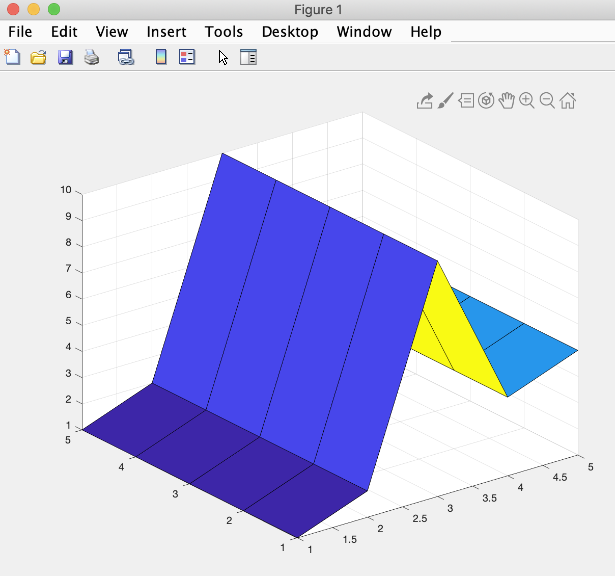
surf(z)into the Interactive Command Window. MATLAB responds by creating a new pop-up window:
that shows a surface plot of the 25 (5 by 5) values. The surface plot is a useful plot in this course because we are modeling phenomenon that are surfaces in nature (the top of land above water is a topography surface and the top of land below water is a bathymetry surface).
As we will see in this class, surfaces can also be somewhat artificial by designating interesting locations within a water column a surface (for example, where the density or temperature of the water is all identical). We can also choose a depth from sea level and create a surface to plot from the values found for an area of water at depth.
Now let's take a look at how we can create a 2-D matrix without invoking the services of MATLAB's meshgrid function.
Go ahead and create a new MATLAB script (as you did in the basic introduction to the MATLAB editor interface). Let's call it surface.m. Type:
x = 100
y = 100
grid = rand(x,y)*.1;
grid(1,1) = 0
surf(grid)
zlim([-5 5])
into the script editor, save the script, and use the Run button to run it.
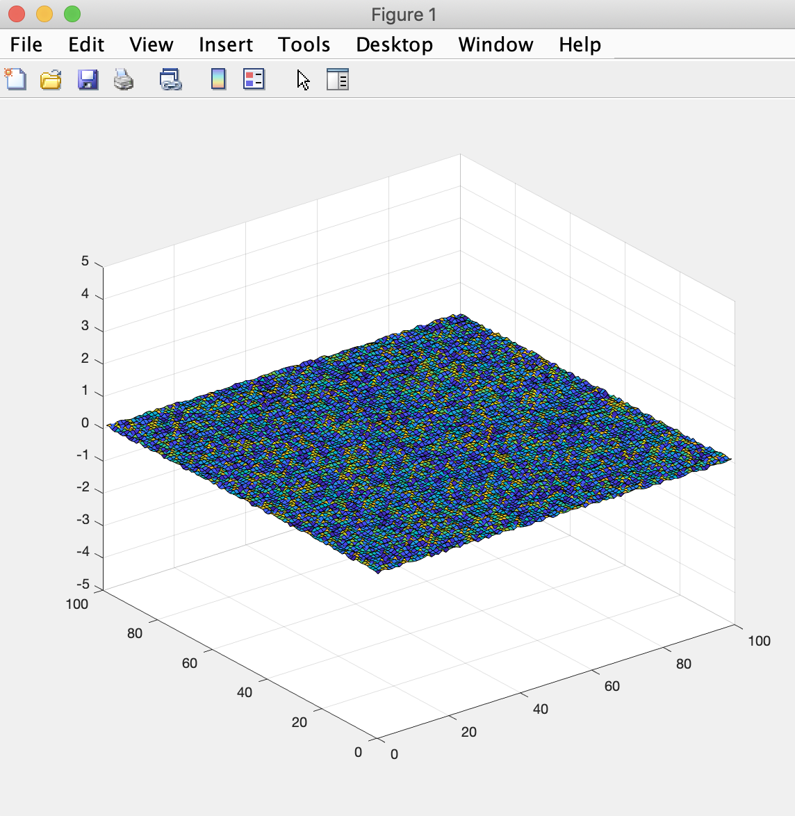
MATLAB responds by creating a new pop-up window:
that plots a surface of 10,000 (100 by 100) values that range from 0 to 0.1
The first two lines of code (x = 100 and y = 100) declare two variables that have a simple value of 100 each.
The third line of code (grid = rand(x,y)*.1;) declares a variable named grid (we named it something useful) that is assigned a 2-D random matrix of 100 by 100 random values that range from 1 to 0.1 (because rand is a MATLAB function that creates floating point values between 0 and 1 (with each of the possible representations getting an equal probability of being chosen).
The fourth line (grid(1,1) = 0) demonstrates how to index a single value within a 2-D matrix (in this case the first element in the array is assigned the value 0, which overwrites whatever random value had been chosen for that value).
The surf function call creates a surface plot of our grid matrix.
And the last line (zlim([-5 5])) tells MATLAB to plot the surface within a vertical extent of -5 to 5 (we'll get used to negative numbers in this class since we'll be investigating phenomena under sea level).
An important take-home lessons here is how we did not have to write any more code to create a 100 x 100 matrix as we would have had to write to create a 5 x 5 matrix. As long as we are reading in values from some data source file (where the data already exists), we can let MATLAB do the heavy lifting of computing on and displaying the data.
Now let's take a look at a different function we will use often for plotting:
Go ahead and create a new MATLAB script (as you did in the basic introduction to the MATLAB editor interface). Let's call it scatter.m. Type:
x = rand(1,100)
y = rand(1,100)
scatter(x,y)
into the script editor, save the script, and use the Run button to run it.
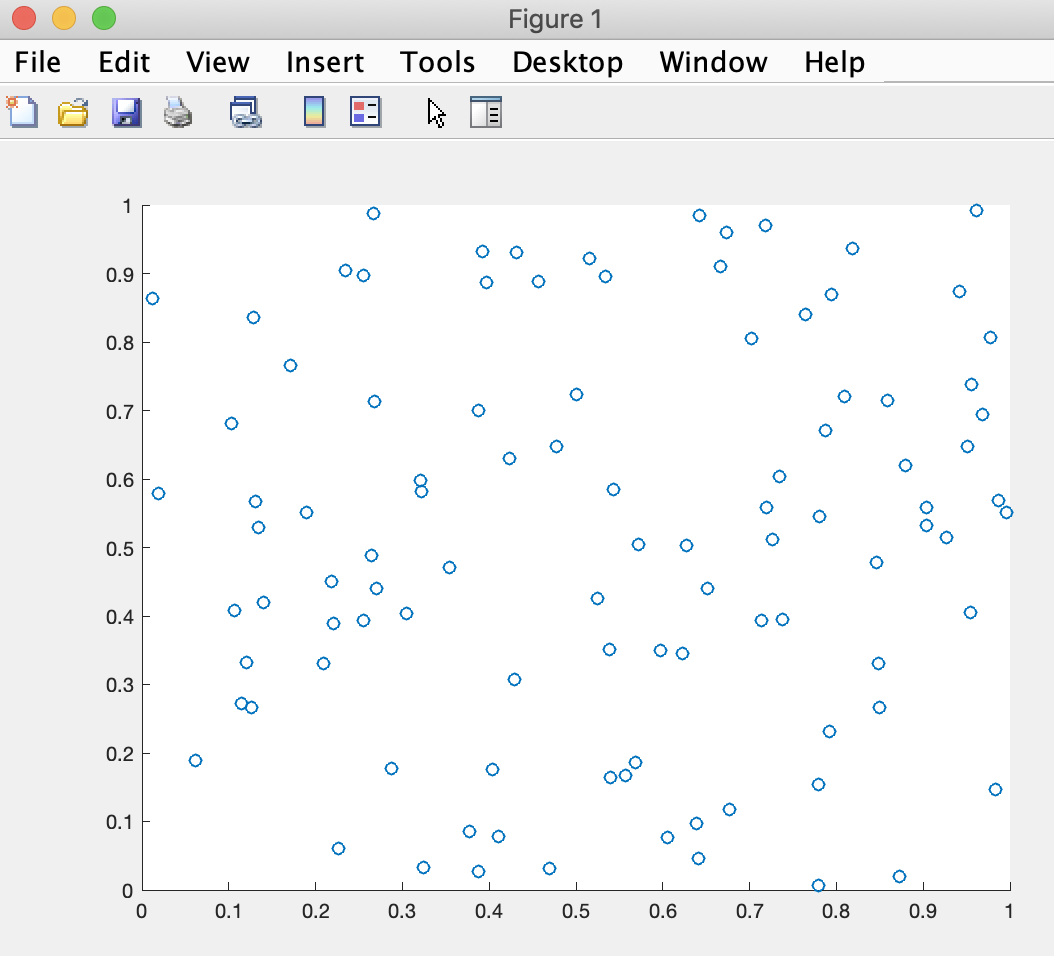
MATLAB responds by creating a new pop-up window:
that plots a scatterplot of one hundred x,y coordinates with x and y each being a random number between 0 and 1.
In this case, there is no 2-D grid. Instead, x and y are each properties of the 100 data points (stored as one-dimensional matrices (vectors)). Conventionally, we expect x to be an independent variable (plotted across the horizontal axis of a plot), and y to be the independent variable (plotted across the horizontal axis of a plot), but there are times to plot data before a causal relationship has been determined (or even hypothesized). We can arbitrarily choose which is x and which is y in that case, and then apply different statistical approaches to look for potential causal relationships.
The important take-home lesson from this module is that sophisticated plotting functions are available in MATLAB, but we have to know the nature of our data and choose an appropriate plotting approach based on the data we want to display. Note that all the functions introduced in this module have hyperlinks to the relevant MATLAB reference pages.
We can dive deeper into any of the concepts suggested herein. We'll dive in deeper together in following modules.
We can of course gain benefit from continuing with more primer modules or reviewing previous ones. They are all linked here for our convenience:
Introduction
Primer 1
Primer 3
Primer 4
Primer 5
Primer 6
Primer 7