

MATLAB Primer - Module 1
Now that you've had a basic introduction to the MATLAB editor interface, we can continue with specific concepts and skills in subsequent modules. In this module, we'll gain exposure to matrices, indices, plotting, and start adding some good program writing techniques.
Recall that we used a linspace function to create values for a variable x. A variable need not be initiated by function, as it can be initiated
by explicit values. For example, if you type:
whereby MATLAB considers variable x a matrix (and in this case also a vector as it is a one-dimensional matrix).
We can create a variable that holds the ages of our three pets:
because the first value in the matrix collection has been set to 9. If we type:
which is the age of our third pet.
Collections are very strict about indexing. If we refer to an index outside of the memory locations contained by the matrix, such as:
Index exceeds the number of array elements (3).
Indexing syntax is used a lot in this class so expect to learn more about it in the following modules. If you want to get a deeper sense of indexing, here's a good resource: Matrix Indexing in MATLAB.
Matrices are useful objects for many mathematical computations. You'll learn many useful operations to perform on matrices in this class. The result of performing mathematical operations on matrices is often one or more matrices. For example, if A and B are both matrices, the line of code:
Go ahead and create a new MATLAB script (as you did in the basic introduction to the MATLAB editor interface). Let's call it matrices.m. Type:
MATLAB shows the result of the script in the Interactive Control Window:
Using the + operator performs mathematical addition on each index of matrix A and matrix B to create the values of matrix C.
Operations on matrices can be done by function name (e.g. cross(A,B)) just as easily as by operator syntax. In fact, cross is one of the functions you will find useful in this class.
As the size and dimensionality of the matrices we use grows, the syntax to perform operations on them need not get more sophisticated. The same goes for functions that let us see the result of operations in useful ways.
Let's turn to a consideration of plotting values in MATLAB.
MATLAB provides a highly capable plot function we can use to turn numbers into pictures. For, example if we add a new line to our script:
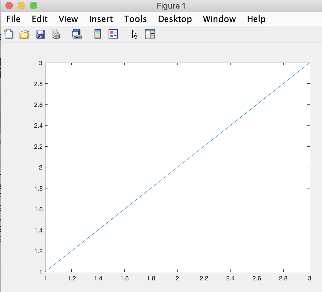
thus creating a line that goes through points (1,1), (2,2), and (3,3).
Whereas if we refer to two matrices as parameters to the plot function:
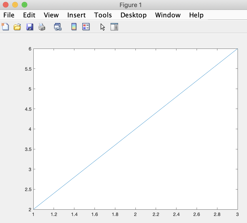
thus creating a line that goes through points (1,2), (2,4), and (3,6).
We will do a lot of plotting in this class. The plots will grow in sophistication and our ability to add labels, legends, and other features for clarity will grow through the use of plotting-related functions that work well together.
If you want to get a deeper sense of plotting, here's a good resource: MATLAB plot reference.
And, of course, plots can get more specialized as they get sophisticated. For example, consider MATLAB's quiver function.
We can use comments in our code to remind us and educate others as to what our intent was at the time of writing our code. We can use the percentage character to create a comment that then does not get run as MATLAB code (but remains in the text file that stores the script). To document better our thinking in the script we've created this module, we can add some comments:
Introduction
Primer 2
Primer 3
Primer 4
Primer 5
Primer 6
Primer 7
x = [0,100,200,300,400,500,600,700,800,900,1000]into the Interactive Command Window. We also immediately get the response:
x =

  Columns 1 through 8

           0         100         200         300         400         500         600         700

  Columns 9 through 11

         800         900        1000

>>
We can create a variable that holds the ages of our three pets:
pet_ages = [9,9,19]and then we can refer to the individual ages by index. MATLAB uses parentheses to refer to an index into a variable that holds a collection of values (and a matrix is just one of many useful collections programmers use). For example, we can refer to the age of the first pet with the syntax:
pet_ages(1)Type that into the Interactive Command Window and MATLAB responds with:
ans =

     9

>>
pet_ages(3)into the Interactive Command Window, MATLAB responds with:
ans =

     19

>>
Collections are very strict about indexing. If we refer to an index outside of the memory locations contained by the matrix, such as:
pet_ages(4)MATLAB will respond with an error message:
Index exceeds the number of array elements (3).
Indexing syntax is used a lot in this class so expect to learn more about it in the following modules. If you want to get a deeper sense of indexing, here's a good resource: Matrix Indexing in MATLAB.
Matrices are useful objects for many mathematical computations. You'll learn many useful operations to perform on matrices in this class. The result of performing mathematical operations on matrices is often one or more matrices. For example, if A and B are both matrices, the line of code:
C = A + Bcreates a variable C that is also a matrix.
Go ahead and create a new MATLAB script (as you did in the basic introduction to the MATLAB editor interface). Let's call it matrices.m. Type:
A = [1,2,3]
B = [2,4,6]
C = A + B
into the script editor, save the script, and use the Run button to run it.
MATLAB shows the result of the script in the Interactive Control Window:
A =

     1     2     3


B =

     2     4     6


C =

     3     6     9

>>
Operations on matrices can be done by function name (e.g. cross(A,B)) just as easily as by operator syntax. In fact, cross is one of the functions you will find useful in this class.
As the size and dimensionality of the matrices we use grows, the syntax to perform operations on them need not get more sophisticated. The same goes for functions that let us see the result of operations in useful ways.
Let's turn to a consideration of plotting values in MATLAB.
MATLAB provides a highly capable plot function we can use to turn numbers into pictures. For, example if we add a new line to our script:
plot(A)and run it, MATLAB generates a plot of a line that uses the values of matrix A in the vertical axis and the index in the horizontal axis:
thus creating a line that goes through points (1,1), (2,2), and (3,3).
Whereas if we refer to two matrices as parameters to the plot function:
plot(A,B)MATLAB generates a plot of a line that uses the values of matrix A in the horizontal axis and the matrix B in the horizontal axis:
thus creating a line that goes through points (1,2), (2,4), and (3,6).
We will do a lot of plotting in this class. The plots will grow in sophistication and our ability to add labels, legends, and other features for clarity will grow through the use of plotting-related functions that work well together.
If you want to get a deeper sense of plotting, here's a good resource: MATLAB plot reference.
And, of course, plots can get more specialized as they get sophisticated. For example, consider MATLAB's quiver function.
We can use comments in our code to remind us and educate others as to what our intent was at the time of writing our code. We can use the percentage character to create a comment that then does not get run as MATLAB code (but remains in the text file that stores the script). To document better our thinking in the script we've created this module, we can add some comments:
A = [1,2,3] %a simple collection of the first three positive integers in succession
B = [2,4,6] %a simple collection of the first three even positive integers in succession
C = A + B   %creates a collection of the first three positive integers exactly divisible by 3
plot(A)     %a plot of a line with slope 1 between 1 and 3
plot(A,B)   %a plot of a line containing the coordinates of A,B for each indexed position
We can of course gain benefit from continuing with more primer modules or reviewing previous ones. They are all linked here for our convenience:
Introduction
Primer 2
Primer 3
Primer 4
Primer 5
Primer 6
Primer 7