
Class on April 5, 2019
Students spent time focusing on implementing their understanding of diffusion-advection process in a model with MATLAB code (as opposed to
Python code, which has a similar one-to-one mapping of functionality:
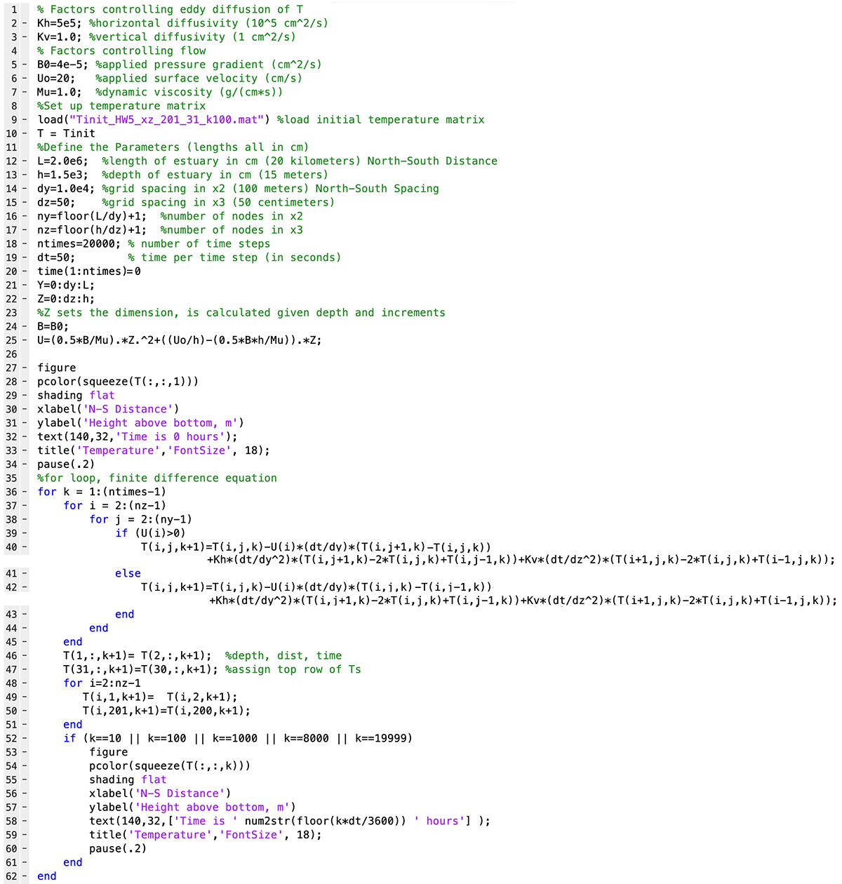
Lines 2 and 3 above set a variable for both a vertical and horizontal thermal diffusivity (the significance of which was discussed on February 18th). Diffusivity affects heat flow energy as reiterated on February 22nd. Lines 5 through 7 set up variables used in the calculation of heat advection discussed in March 4th's class. Line 9 sets up the initial temperature data for the parcels used in the model (by loading in an external file). The full 2-D initialization array can be seen in the text file here.
Line 22 sets up variable Z as a series of equally distributed depths over the depth of the water column. Lines 24 and 25 set up advection values for each depth using the equation discussed in March 25th's class. The MATLAB implementation here does not declare a function for use as a subroutine. Instead the calculation is done inline within the nested loops that start on line 36. Lines 39 through 43 make sure the model remains stable by calculating the effect of advection depending on whether the flow is coming toward or away from the parcel. The first sub-line of lines 40 and 42 calculate the effect of advection by taking into account neighboring parcels (horizontally) while the second sub-line of lines 40 and 42 calculate the effect of diffusion by taking in to account neighboring parcels (horizontally and vertically).
Temperatures for each parcel in the model are calculated once per timestep (for all parcels in the simulation according to the discussions held on March 18th). Line 36 begins the 3-D nesting of iterator variables (time, depth, and length). Code for a plot of the temperatures for the timesteps is included in each timestep run (as opposed to the Python that plotted the data after all timesteps were run — which made the run available for other numerical processing post-looping). Using variables in plotting was described on March 18th as well.
A screen capture of three timesteps (100, 1000, and 19999) does a nice job of showing off the spreading of temperature over time (creating a stratified effect by depth):
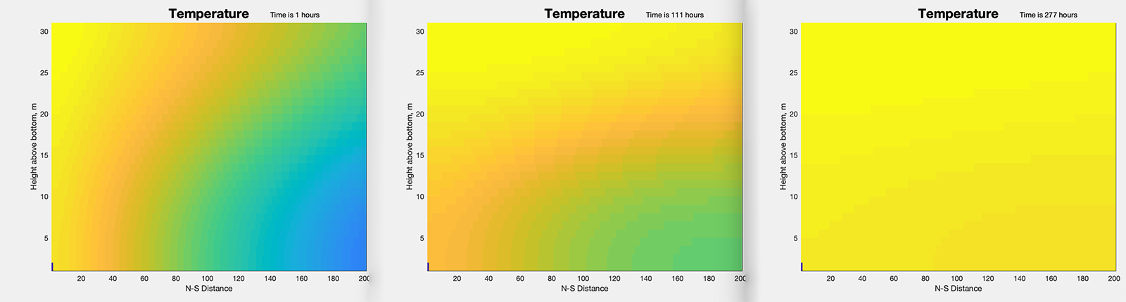
Students were asked to make sure they understood the MATLAB code before attempting to enhance it for chemical transport.
Lines 2 and 3 above set a variable for both a vertical and horizontal thermal diffusivity (the significance of which was discussed on February 18th). Diffusivity affects heat flow energy as reiterated on February 22nd. Lines 5 through 7 set up variables used in the calculation of heat advection discussed in March 4th's class. Line 9 sets up the initial temperature data for the parcels used in the model (by loading in an external file). The full 2-D initialization array can be seen in the text file here.
Line 22 sets up variable Z as a series of equally distributed depths over the depth of the water column. Lines 24 and 25 set up advection values for each depth using the equation discussed in March 25th's class. The MATLAB implementation here does not declare a function for use as a subroutine. Instead the calculation is done inline within the nested loops that start on line 36. Lines 39 through 43 make sure the model remains stable by calculating the effect of advection depending on whether the flow is coming toward or away from the parcel. The first sub-line of lines 40 and 42 calculate the effect of advection by taking into account neighboring parcels (horizontally) while the second sub-line of lines 40 and 42 calculate the effect of diffusion by taking in to account neighboring parcels (horizontally and vertically).
Temperatures for each parcel in the model are calculated once per timestep (for all parcels in the simulation according to the discussions held on March 18th). Line 36 begins the 3-D nesting of iterator variables (time, depth, and length). Code for a plot of the temperatures for the timesteps is included in each timestep run (as opposed to the Python that plotted the data after all timesteps were run — which made the run available for other numerical processing post-looping). Using variables in plotting was described on March 18th as well.
A screen capture of three timesteps (100, 1000, and 19999) does a nice job of showing off the spreading of temperature over time (creating a stratified effect by depth):
Students were asked to make sure they understood the MATLAB code before attempting to enhance it for chemical transport.