

Class on February 22 2019
Chris performed the energy equation expansion in preparation for discussing a three node heat flow progression:

He gave a handout for students to work on in teams of three:
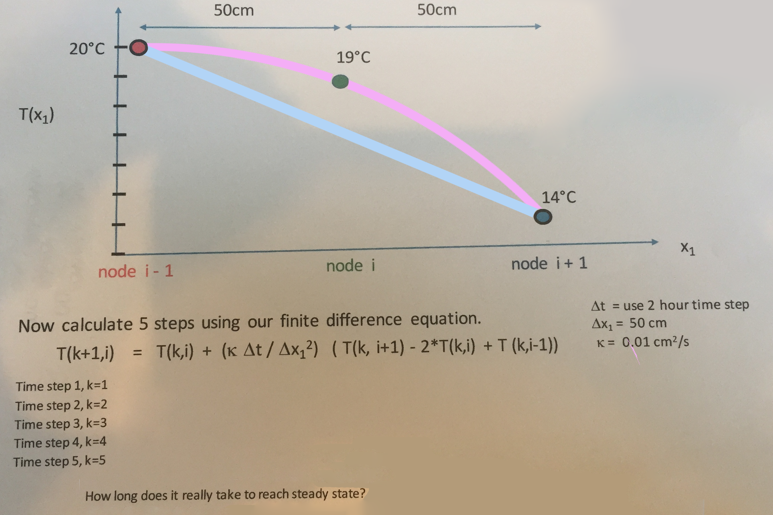
and walked through how the heat flow relationship progresses from the pink curve to the blue straight line over time (decreasing curvature with time). He used the visual prop of a curved ruler to get students to make comments about the relative magnitude of various components in relevant equations.
Chris explained the relationship of curvature (a second-order concept):
δ2T/(δx1)2
to the linear δT/δt (a first-order concept)
and reminded us that δT/δt gets multiplied by kappa (which has a typical value of .01), which means changes in the temperature function curvature have a dampered effect on change in temperature.
Chris then asked students about the significance of:
δ3T/(δx1)3
which is the change in curvature in the x1 direction
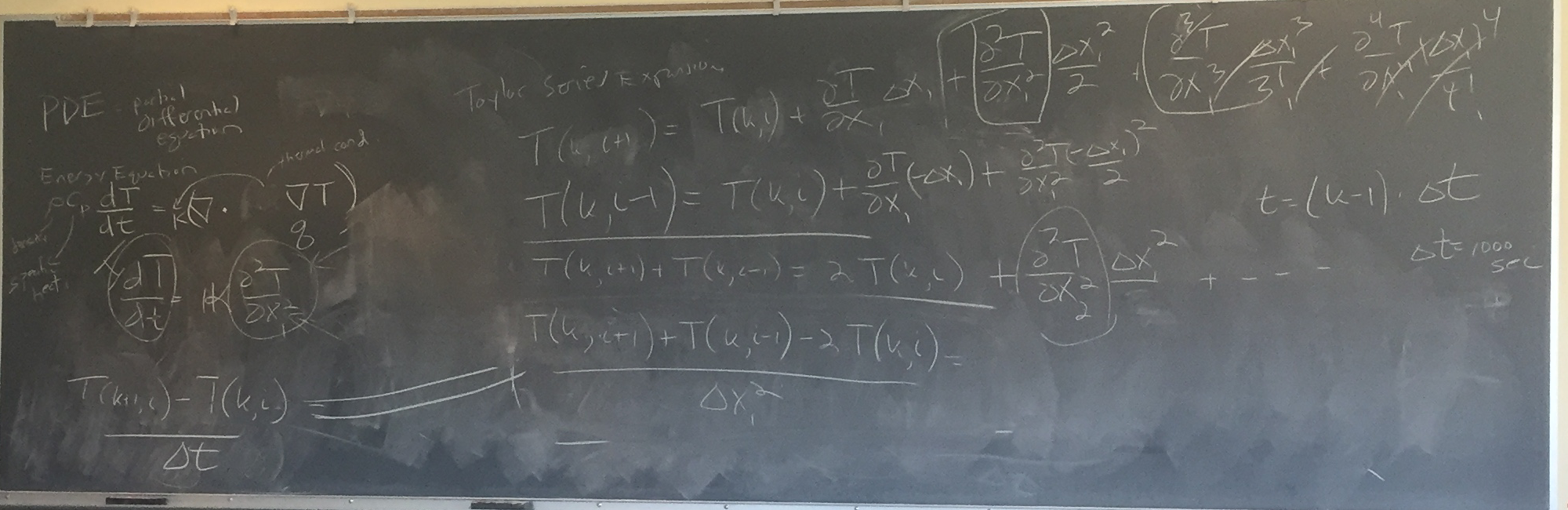
Chris then went over how the Taylor Expansion of all the n-order differentials lets us get from a Partial Differential Equation (PDE) to a Finite Difference Equation (FDE) which is useful because the FDE can then be solved numerically. The Taylor expansion becomes:
δT/δx1 * △x1 + δ2T/(δx1)2 * △x12/2 + δ3T/(δx1)3 * △x13/3 + δ4T/(δx1)4 * △x14/4 + δ5T/(δx1)5 * △x15/5 +
[...] + δnT/(δx1)n * △x1n/n
as seen in the upper right of the blackboard here:

Chris showed how when one decreases delta time to be small enough, the higher order terms (after curvature) become immaterial and can be considered irrelevant.
He reminded students that the rate of change in Temperature decreases over time (the curve in the middle of the blackboard above)
Then he solved for the T(k+1, i) — where k is the node (distance in x1) and i is the timestep (see the blackboard above).
Solving involves adding up positive and negative components of the Taylor series, where the odd terms (1, 3, 5, etc.) cancel out, but the even terms (2, 4, 6, etc.) double their magnitude (since negative numbers raised to even powers become positive).
The rearranging of terms leads to the equation used in homework assignment #4 for determining the temperature of each node at each timestep (based on the temperature at the previous timestep):
To get a better intuition of how the equation works, Chris had nine students stand to create a two-dimensional array of 3x3 where the time dimension lined up from the back of the room (k=1) towards the front of the room (k=3) and the nodes lined up from left to right (when facing the front of the room). Students stood at the height of the temperature for their node at their time and Chris had them raise their hands when their k,i position was being referenced in the equation:
Thinking of those student positions could help when thinking through the MATLAB (or Python) code required for calculating all T(k,i) forecasts given fixed values for T(1,1), T(2,1), T(3,1), T(1,3), T(2,3), and T(3,3) — and a known value for T(1, 2)
Chris wrote MATLAB code for a nested for loop on the blackboard:
Students were asked to continue working on homework assignment #4 and to ask for help on their code early and often when needed.
He gave a handout for students to work on in teams of three:
and walked through how the heat flow relationship progresses from the pink curve to the blue straight line over time (decreasing curvature with time). He used the visual prop of a curved ruler to get students to make comments about the relative magnitude of various components in relevant equations.
Chris explained the relationship of curvature (a second-order concept):
δ2T/(δx1)2
to the linear δT/δt (a first-order concept)
and reminded us that δT/δt gets multiplied by kappa (which has a typical value of .01), which means changes in the temperature function curvature have a dampered effect on change in temperature.
Chris then asked students about the significance of:
δ3T/(δx1)3
which is the change in curvature in the x1 direction
Chris then went over how the Taylor Expansion of all the n-order differentials lets us get from a Partial Differential Equation (PDE) to a Finite Difference Equation (FDE) which is useful because the FDE can then be solved numerically. The Taylor expansion becomes:
δT/δx1 * △x1 + δ2T/(δx1)2 * △x12/2 + δ3T/(δx1)3 * △x13/3 + δ4T/(δx1)4 * △x14/4 + δ5T/(δx1)5 * △x15/5 +
[...] + δnT/(δx1)n * △x1n/n
as seen in the upper right of the blackboard here:
Chris showed how when one decreases delta time to be small enough, the higher order terms (after curvature) become immaterial and can be considered irrelevant.
He reminded students that the rate of change in Temperature decreases over time (the curve in the middle of the blackboard above)
Then he solved for the T(k+1, i) — where k is the node (distance in x1) and i is the timestep (see the blackboard above).
Solving involves adding up positive and negative components of the Taylor series, where the odd terms (1, 3, 5, etc.) cancel out, but the even terms (2, 4, 6, etc.) double their magnitude (since negative numbers raised to even powers become positive).
The rearranging of terms leads to the equation used in homework assignment #4 for determining the temperature of each node at each timestep (based on the temperature at the previous timestep):
To get a better intuition of how the equation works, Chris had nine students stand to create a two-dimensional array of 3x3 where the time dimension lined up from the back of the room (k=1) towards the front of the room (k=3) and the nodes lined up from left to right (when facing the front of the room). Students stood at the height of the temperature for their node at their time and Chris had them raise their hands when their k,i position was being referenced in the equation:
Thinking of those student positions could help when thinking through the MATLAB (or Python) code required for calculating all T(k,i) forecasts given fixed values for T(1,1), T(2,1), T(3,1), T(1,3), T(2,3), and T(3,3) — and a known value for T(1, 2)
Chris wrote MATLAB code for a nested for loop on the blackboard:
for k = 2:nk
  for i = 2:ni
and the derived T(k, i) equation would be used to compute each k,i pair within the nested for loops.
Students were asked to continue working on homework assignment #4 and to ask for help on their code early and often when needed.