

Class on February 18 2019
Chris warmed us by reminding us of where we are on our progress with the conservation of energy equation (Fourier's Law):
ρ * cp * dT/dt = ▽ · q + H0 + work
He reviewed everything we had done last class: a kinesthetic exercise of simulating heat flow in a body of water by using the room as the body, a small bin as the parcel, and pipes for the flow from four directions (no depth).
We had the usual math expansion competition between two teams doing a ▽ · q expansion on the blackboard — trying to get faster at it yet.
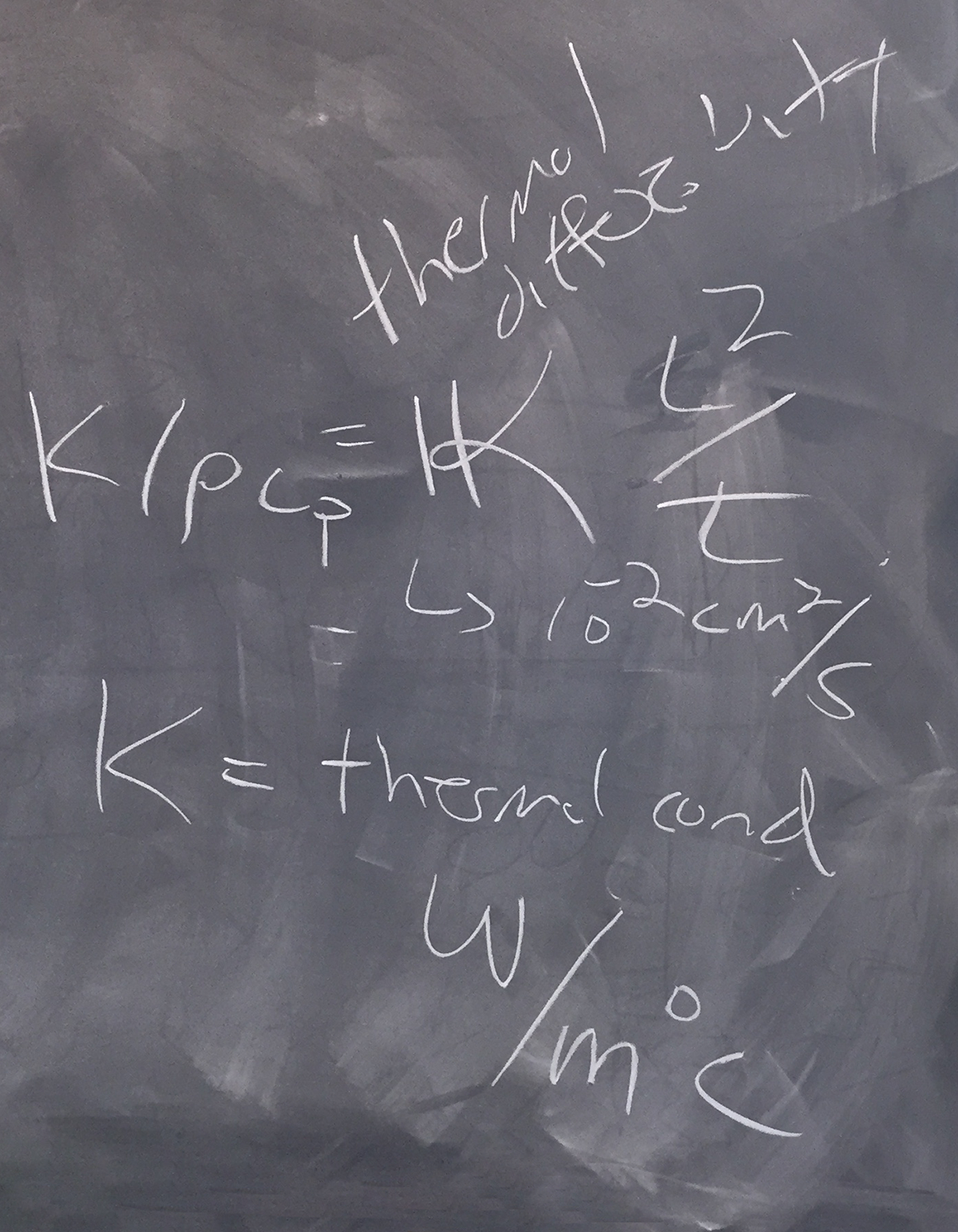
Chris presented the math we had used last class, but lingered on a discussion of the difference between
K (which, as thermal conductivity, is described in terms of watts/(meter * °C)) and Kappa, as thermal diffusivity, which is described in units cm2/second). The relationship between the two can be considered as:
Chris then showed the ▽ · q expansion as relevant to K and Kappa expansions (starting with q = K/(ρ * cp)):
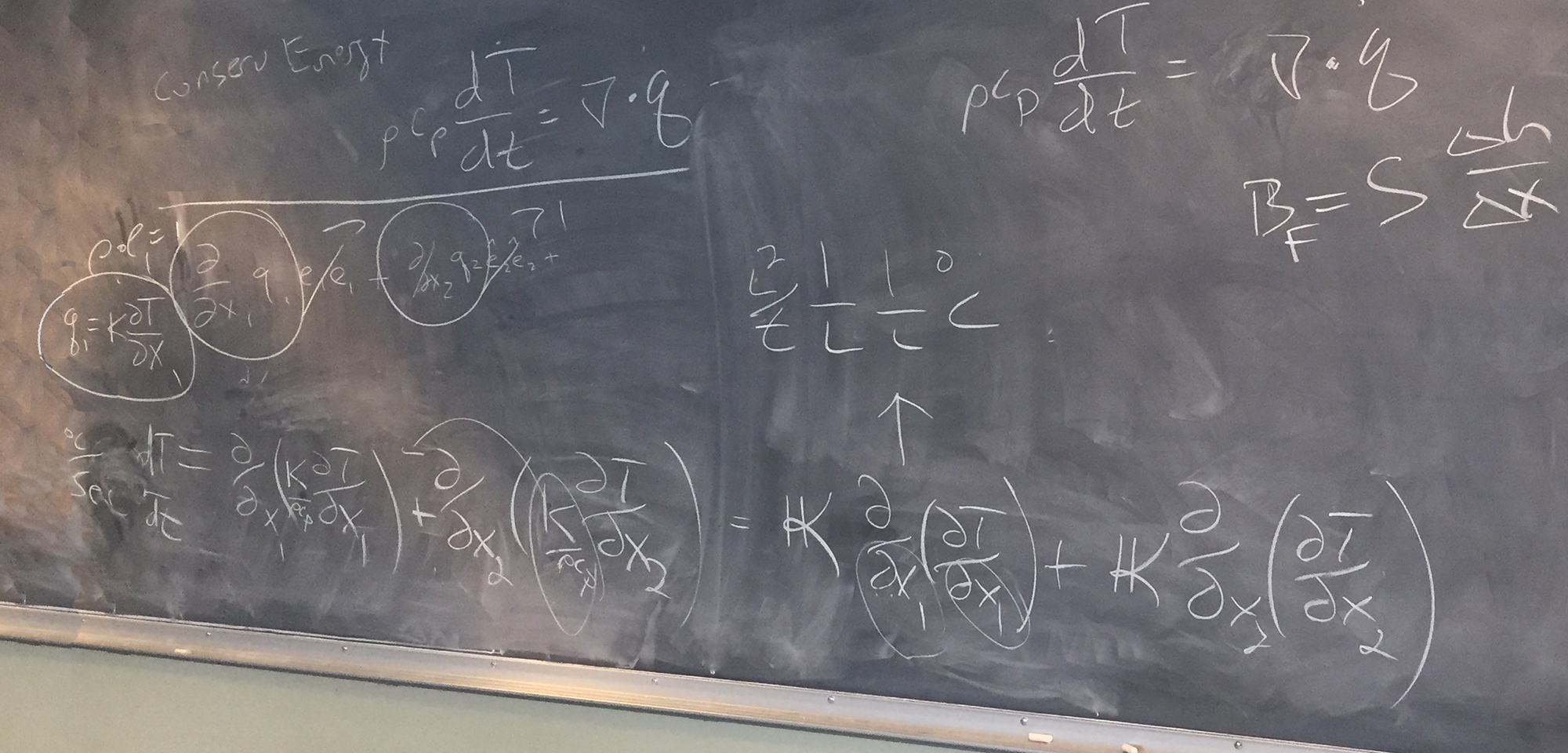
and then he derived the relevant equation we used in the end of period exercise last class:
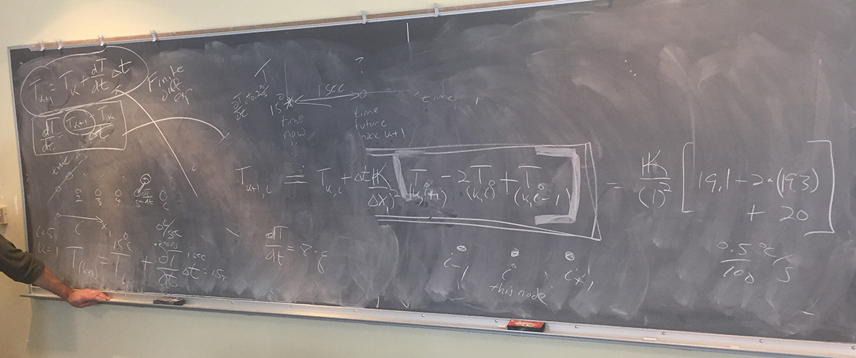
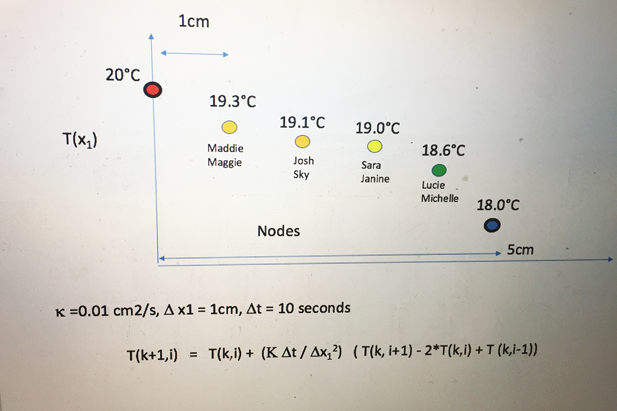
Chris then presented the class a parcel chain situation and broke the students into teams of two to calculate the heat flow for each node in the chain:
Bruce was asked to create a heat flow calculations notebook using the Jupyter Python notebook technology mentioned in class.
The notebook can be downloaded here (just right-mouse click on the link and choose Save Link As to save the default native notebook format on your hard drive).
Using a notebook makes it easy to calculate as many iterations over time as you'd want to make (the image here shows an example using 130 iterations):
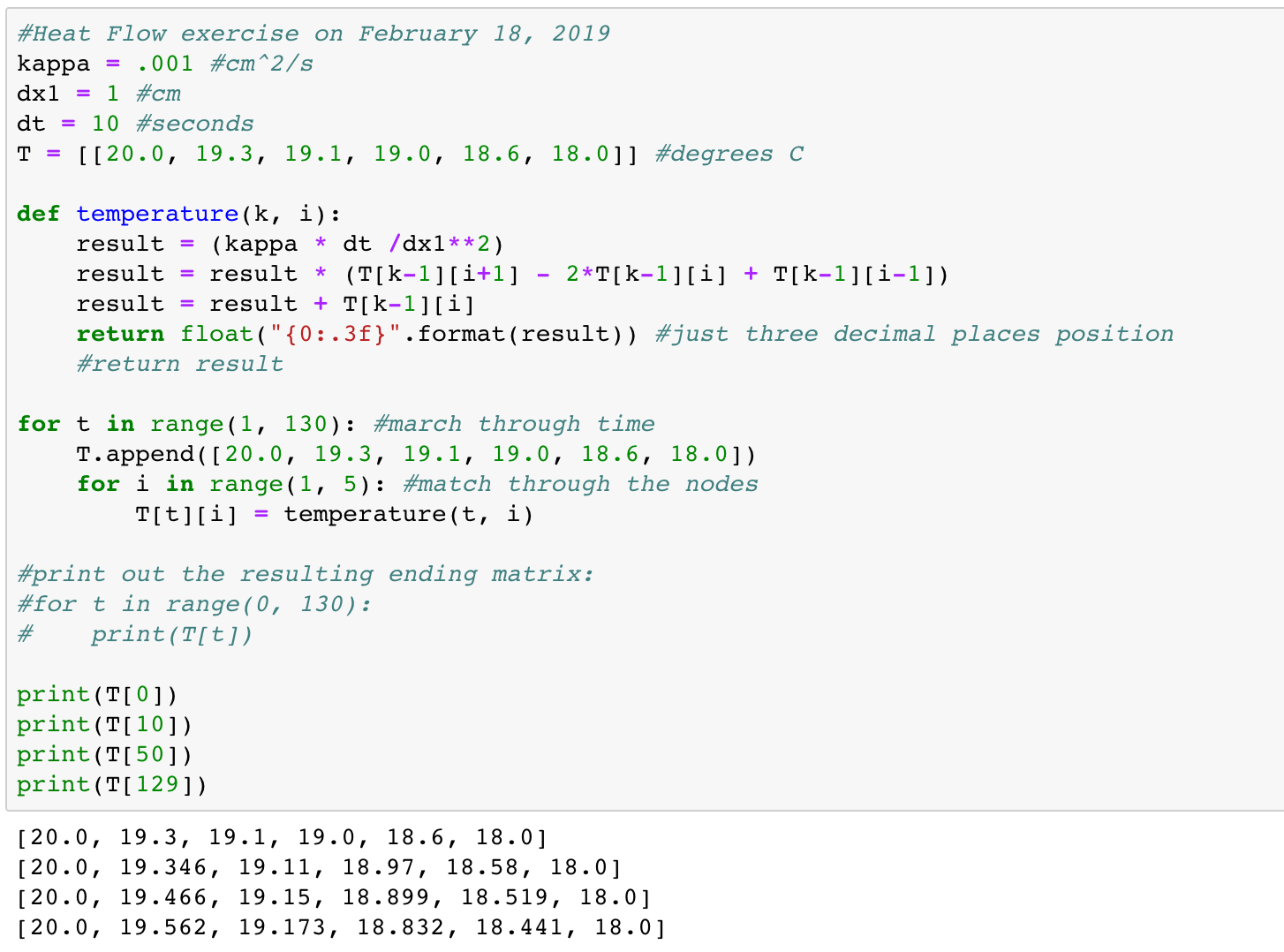
Note how the three relevant coefficients are created up front. A two-dimensional array (nodes in rows, time in columns) is declared next.
The calculation of heat flow per node is encapsulated in a temperature() function that does the calculation in three steps (passing in time and node as parameters).
The for loops afford the time iteration process for each node (filling out a new row in the array for each timestep).
As Bruce verified the code reached a stable (equilibrium) state at timestep number 129 (using three decimals of precision in the calculation results), he printed out some representative timesteps in the progression (the same he plotted below).
The plotting code uses typical Python packages for doing plots and numerical compuation (numpy, matplotlib, and math):
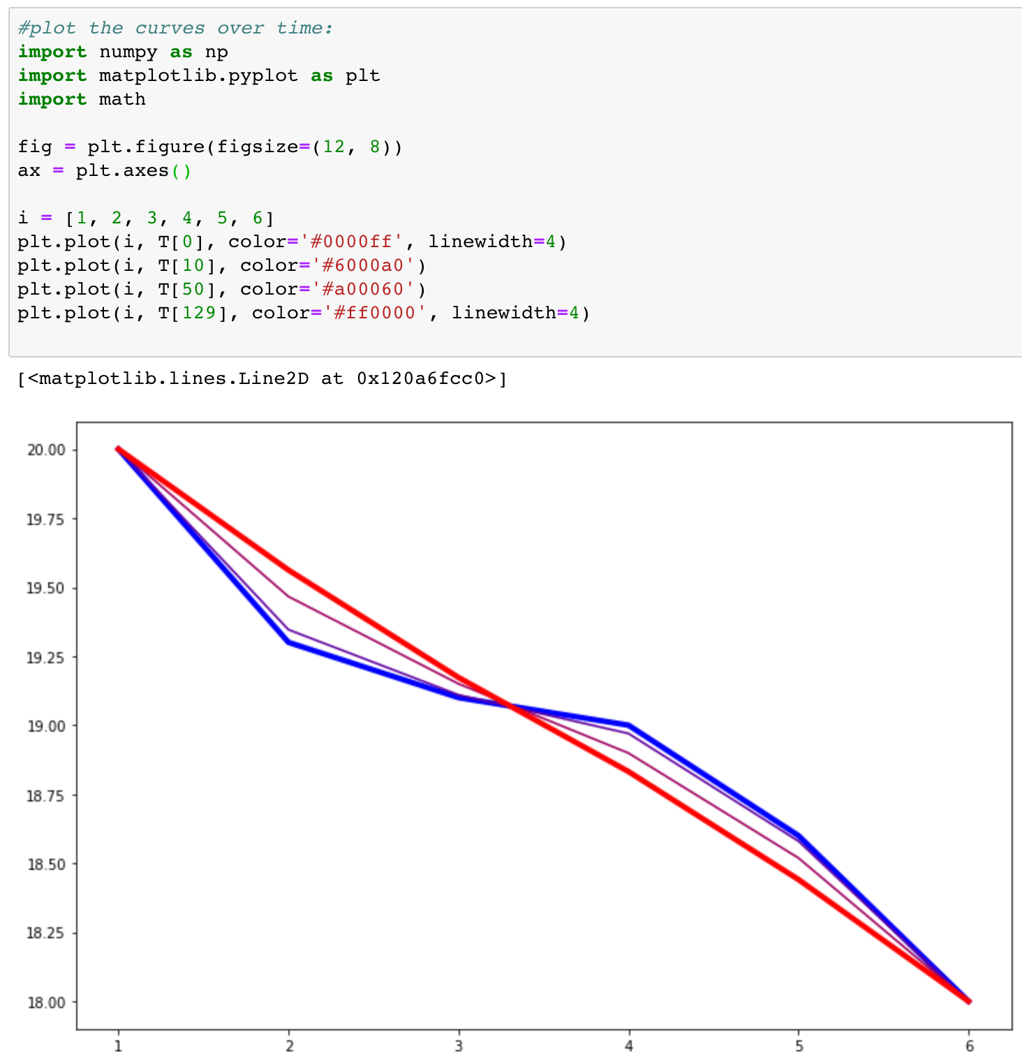
The code sets up a new figure, defines the axes (which can then be labeled later), creates an array of node identifiers, and then plots starting conditions (blue), timestep 10 (purple), timestep 50 (violet), and timestep 129 (red) to show how the heat converges on a straight line between nodes.
Chris asked students to continue to do calculations until the process was familiar. He also suggested the next homework assignment would be distributed by e-mail shortly.
ρ * cp * dT/dt = ▽ · q + H0 + work
He reviewed everything we had done last class: a kinesthetic exercise of simulating heat flow in a body of water by using the room as the body, a small bin as the parcel, and pipes for the flow from four directions (no depth).
We had the usual math expansion competition between two teams doing a ▽ · q expansion on the blackboard — trying to get faster at it yet.
Chris presented the math we had used last class, but lingered on a discussion of the difference between
K (which, as thermal conductivity, is described in terms of watts/(meter * °C)) and Kappa, as thermal diffusivity, which is described in units cm2/second). The relationship between the two can be considered as:
Chris then showed the ▽ · q expansion as relevant to K and Kappa expansions (starting with q = K/(ρ * cp)):
and then he derived the relevant equation we used in the end of period exercise last class:
Chris then presented the class a parcel chain situation and broke the students into teams of two to calculate the heat flow for each node in the chain:
Bruce was asked to create a heat flow calculations notebook using the Jupyter Python notebook technology mentioned in class.
The notebook can be downloaded here (just right-mouse click on the link and choose Save Link As to save the default native notebook format on your hard drive).
Using a notebook makes it easy to calculate as many iterations over time as you'd want to make (the image here shows an example using 130 iterations):
Note how the three relevant coefficients are created up front. A two-dimensional array (nodes in rows, time in columns) is declared next.
The calculation of heat flow per node is encapsulated in a temperature() function that does the calculation in three steps (passing in time and node as parameters).
The for loops afford the time iteration process for each node (filling out a new row in the array for each timestep).
As Bruce verified the code reached a stable (equilibrium) state at timestep number 129 (using three decimals of precision in the calculation results), he printed out some representative timesteps in the progression (the same he plotted below).
The plotting code uses typical Python packages for doing plots and numerical compuation (numpy, matplotlib, and math):
The code sets up a new figure, defines the axes (which can then be labeled later), creates an array of node identifiers, and then plots starting conditions (blue), timestep 10 (purple), timestep 50 (violet), and timestep 129 (red) to show how the heat converges on a straight line between nodes.
Chris asked students to continue to do calculations until the process was familiar. He also suggested the next homework assignment would be distributed by e-mail shortly.