

Class on March 18 2019
Chris put the students into teams based on their coding prowess demonstrated in homeworks 1-4. The teams worked to extract the key elements of coding
for a 1-D heat flow model, in order to see the path towards writing model code for 2-D, 3-D, or any N-D phenomenon.
Students extrapolated upon the coin and block exercise used to prep homework #4:
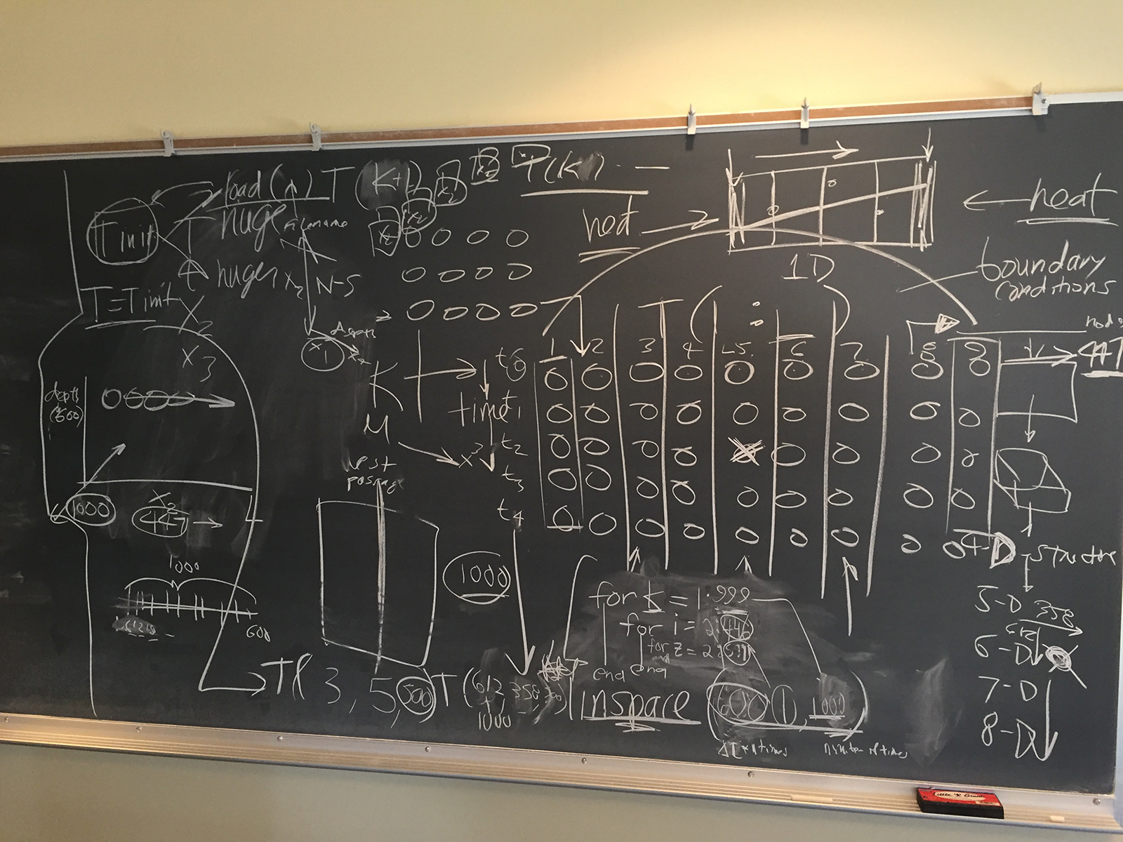
First of interest was the T() syntax that described a temperature value in any temperature data set. For Homework 4a, T ranged as T(1:9, 1:5) whereby T(3,5) represented the temperature during the third timestep of the fifth node (represented in the homework problem from left to right).
To add another dimension to T, a third range could be added such that:
T(1:9, 1:5, 1:4)
would create a memory model that could manage 9 nodes across a length L, across 5 timesteps, with 4 different depths. Once the syntax is familiar, the size of the memory model doesn't matter for declaring a memory model:
T(358,500,612) would represent the temperature of the 358th node along L, at the 500th timestep, at the 612th depth, but of course in terms of Homework 5's consideration of modeling eddies, L is a more dynamic variable than depth and the memory model would probably have more length detail than depth. That would refer to a single temperature scalar from a memory model of T(1:447,1:600,1:1000)
The memory model of a variable of interest advises the formation of the for loop that is used to process it. So in the case of the 1-D node code (where time is a second dimension):
The other automation assistance discussed was the linspace() function that MATLAB provides (and Python provides via the numpy package). When we want to create a scatter plot of two variables in an analysis, we need to have the same number of values for each variable. So, when we want to plot temperature versus any other variable, we can get all the temperatures over time by requesting the full range with a colon (:) as syntax:
T(358,:,612)
but we need a variable for time to plot against the temperature values. The linspace() function would allow us to create and initiate a variable:
x = linspace(600, 1, 600)
which starts at 1 (the middle parameter), continues to 600 (the first parameter) and creates a linear progression of 600 values between them (the third parameter). We can now plot T(358,:,612) versus x (you can create an intermediary variable y with y = T(358,:,612) if you want to self-document your plot(x,y) syntax).
When used with time, the first parameter can be set to delta time * the number of timesteps (such as in homework 4b, where each timestep is 1000 seconds).
Note the colon syntax can extract temperature over time no matter how many dimensions are in the memory model.
Also note the for loops assume a strategy of calculating the current T from T at k-1 (Chris often uses a strategy of calculating T at k+1 from the current T — in that case the k variable only should run run to number of timesteps minus 1).
To drive the point home, we can consider a 3-D node model (where time is then a fourth dimension):
T(1:447,1:600,1:1000,1:20)
Students were asked to continue to work on Homework #5, but with the coding knowledge shared in class today in mind. A useful goal is to write the code with variables and syntax that let you grow the data tremendously (for example, by increasing the resolution of the model) without having to do much to the code (just change the numbers associated with the syntax above, or copy and paste code to expand dimensionality).
Students extrapolated upon the coin and block exercise used to prep homework #4:
First of interest was the T() syntax that described a temperature value in any temperature data set. For Homework 4a, T ranged as T(1:9, 1:5) whereby T(3,5) represented the temperature during the third timestep of the fifth node (represented in the homework problem from left to right).
To add another dimension to T, a third range could be added such that:
T(1:9, 1:5, 1:4)
would create a memory model that could manage 9 nodes across a length L, across 5 timesteps, with 4 different depths. Once the syntax is familiar, the size of the memory model doesn't matter for declaring a memory model:
T(358,500,612) would represent the temperature of the 358th node along L, at the 500th timestep, at the 612th depth, but of course in terms of Homework 5's consideration of modeling eddies, L is a more dynamic variable than depth and the memory model would probably have more length detail than depth. That would refer to a single temperature scalar from a memory model of T(1:447,1:600,1:1000)
The memory model of a variable of interest advises the formation of the for loop that is used to process it. So in the case of the 1-D node code (where time is a second dimension):
for k=1:5
   for i=2:8
the 5 is the upper bounds on the timestep dimension, and the 8 is one less than the upper bounds on node number (nodes 1 and 9 do not need updating since they are boundary conditions that stay the same throughout the model process). To create the for loops for our larger 2-D node analysis (where time is a third dimension) we write:
for k=1:600
   for i=2:446
      for z=2:999
since the memory model is T(1:447,1:600,1:1000).
The other automation assistance discussed was the linspace() function that MATLAB provides (and Python provides via the numpy package). When we want to create a scatter plot of two variables in an analysis, we need to have the same number of values for each variable. So, when we want to plot temperature versus any other variable, we can get all the temperatures over time by requesting the full range with a colon (:) as syntax:
T(358,:,612)
but we need a variable for time to plot against the temperature values. The linspace() function would allow us to create and initiate a variable:
x = linspace(600, 1, 600)
which starts at 1 (the middle parameter), continues to 600 (the first parameter) and creates a linear progression of 600 values between them (the third parameter). We can now plot T(358,:,612) versus x (you can create an intermediary variable y with y = T(358,:,612) if you want to self-document your plot(x,y) syntax).
When used with time, the first parameter can be set to delta time * the number of timesteps (such as in homework 4b, where each timestep is 1000 seconds).
Note the colon syntax can extract temperature over time no matter how many dimensions are in the memory model.
Also note the for loops assume a strategy of calculating the current T from T at k-1 (Chris often uses a strategy of calculating T at k+1 from the current T — in that case the k variable only should run run to number of timesteps minus 1).
To drive the point home, we can consider a 3-D node model (where time is then a fourth dimension):
T(1:447,1:600,1:1000,1:20)
which would require for loops of:
for k=1:600
   for i=2:446
      for z=2:999
         for j=1:19
whereby the code writer would have to be sure to use the k, i, z, and j variables carefully (for their known representations in the data). The order
of the ranges within T() can be in any order, but there are conventions used among modelers within their communities.
Students were asked to continue to work on Homework #5, but with the coding knowledge shared in class today in mind. A useful goal is to write the code with variables and syntax that let you grow the data tremendously (for example, by increasing the resolution of the model) without having to do much to the code (just change the numbers associated with the syntax above, or copy and paste code to expand dimensionality).