
Class on April 1, 2019
Students spent the class investigating the Homework 6 code with the intent of tying the code solution to the mathematical framework supporting its logic. The homework
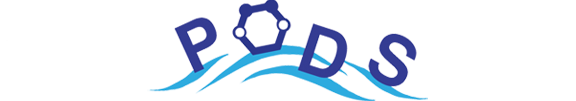
creates a model of temperature change for parcels of water in the March 22nd's class scenario. That scenario dictates the variables in
lines 1 through 6 here:
Lines 7 and 8 above set a variable for both a vertical and horizontal thermal diffusivity (the significance of which was discussed on February 18th). Diffusivity affects heat flow energy as reiterated on February 22nd. Lines 9 through 11 set up variables used in the calculation of heat advection discussed in March 4th's class. Line 14 sets up the initial temperature data for the parcels used in the model. The full 2-D initialization array can be seen in the text file here.
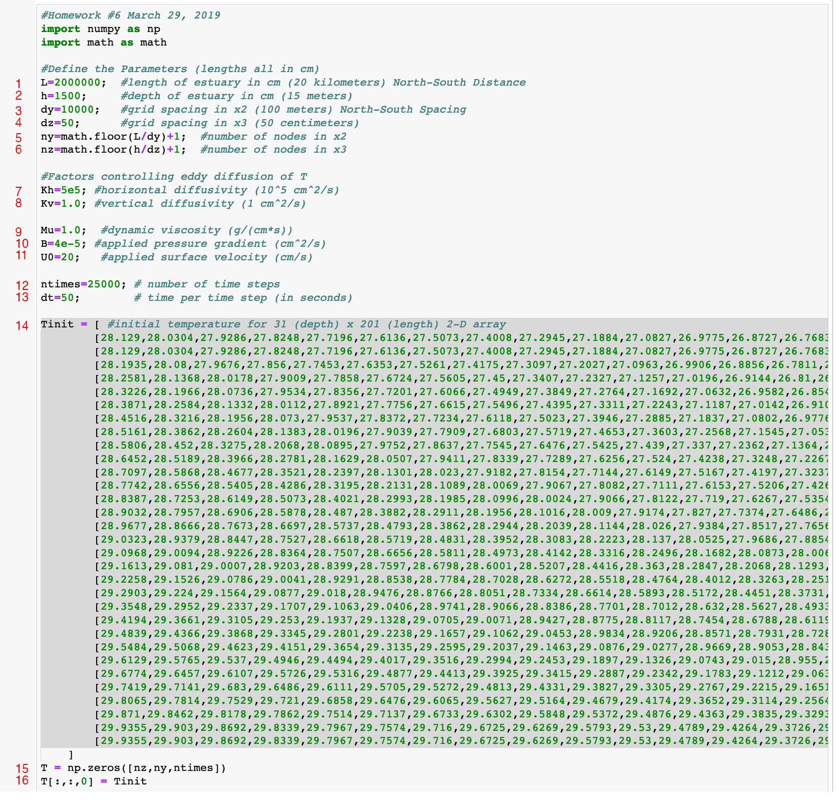
The code continues by marching the diffusion-advection model forward through time:
Line 1 immediately above sets up variable Z as a series of equally distributed depths over the depth of the water column. Lines 2 and 3 set up advection values for each depth using the equation discussed in March 25th's class. Python enables the use of functions through the def keyword as seen in line 4 (lines 5 through 12 contain the body of the function, identified through their identation). Lines 6 through 9 make sure the model remains stable by calculating the effect of advection depending on whether the flow is coming toward or away from the parcel. Lines 10 and 11 calculate the effect of diffusion by taking in to account neighboring parcels (horizontally in line 10 and vertically in line 11).
Once the function is set up, the code uses it as a subroutine once per timestep (but for all parcels in the simulation according to the discussions held on March 18th). Line 13 begins the 3-D nesting of iterator variables (time, depth, and length). Code for a plot of the temperatures for the starting condition starts at the 14 and continues to the bottom of the page. The logic for plotting in two dimensions instead of one follows from the discussion on March 18th as well.
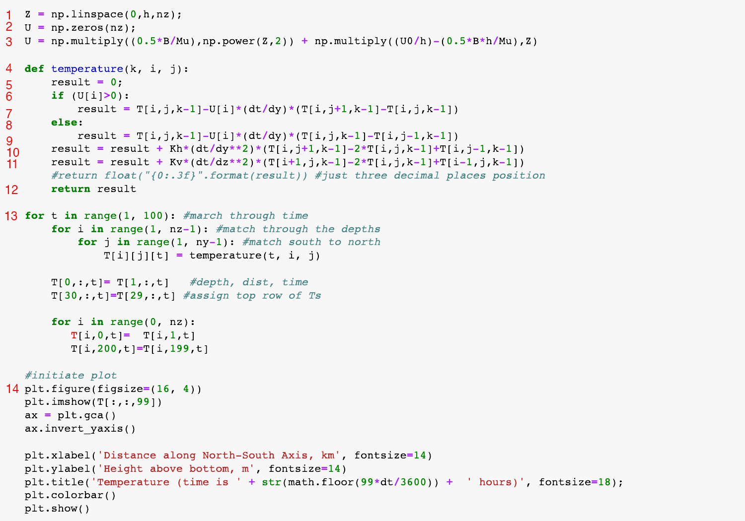
The code below creates a plot for any timestep (the 9999 on the second line and third from last line refers to the 10000th timestep — just change that value to get a plot for any timestep. Plots for timestep 99, 999, and 9999 are shown here:
which does a nice job of showing off the spreading of temperature over time (creating a stratified effect by depth).
Lines 7 and 8 above set a variable for both a vertical and horizontal thermal diffusivity (the significance of which was discussed on February 18th). Diffusivity affects heat flow energy as reiterated on February 22nd. Lines 9 through 11 set up variables used in the calculation of heat advection discussed in March 4th's class. Line 14 sets up the initial temperature data for the parcels used in the model. The full 2-D initialization array can be seen in the text file here.
The code continues by marching the diffusion-advection model forward through time:
Line 1 immediately above sets up variable Z as a series of equally distributed depths over the depth of the water column. Lines 2 and 3 set up advection values for each depth using the equation discussed in March 25th's class. Python enables the use of functions through the def keyword as seen in line 4 (lines 5 through 12 contain the body of the function, identified through their identation). Lines 6 through 9 make sure the model remains stable by calculating the effect of advection depending on whether the flow is coming toward or away from the parcel. Lines 10 and 11 calculate the effect of diffusion by taking in to account neighboring parcels (horizontally in line 10 and vertically in line 11).
Once the function is set up, the code uses it as a subroutine once per timestep (but for all parcels in the simulation according to the discussions held on March 18th). Line 13 begins the 3-D nesting of iterator variables (time, depth, and length). Code for a plot of the temperatures for the starting condition starts at the 14 and continues to the bottom of the page. The logic for plotting in two dimensions instead of one follows from the discussion on March 18th as well.
The code below creates a plot for any timestep (the 9999 on the second line and third from last line refers to the 10000th timestep — just change that value to get a plot for any timestep. Plots for timestep 99, 999, and 9999 are shown here:
which does a nice job of showing off the spreading of temperature over time (creating a stratified effect by depth).