We have installed the Anaconda program and explored the use of Jupyter notebooks. Our work so far has entailed using the Python language to perform data manipulation and visualization. Many of us have used Python for this purpose for years. Python grew rapidly as a popular data manipulation language that processed inputs, internals, and outputs to scientific models, even allowing for models written in other languages to be wrapped by Python (see SWIG, for example) for easy data infusion and reporting purposes. Python interprets statements one at a time where as many scientific models are written on sophisticated platforms that run code in other ways (parallel, instead of sequential, processing included).

Before the coordinated notebooking facilities, python could be invoked in two popular ways (which will still work fine today on a machine where the Anaconda application suite of tools have been loaded. Below are two examples of using traditional Python means to pursue what we pursued on February 1st in class:

Running Python commands interactively in a Terminal application

Operating systems provide applications for interacting with the control of a computer through typed commands. On the Mac OS (and most flavors of Linux), there is an application called Terminal (as seen below). Within the Windows OS, there is an application called Command (or cmd or Command Prompt). Launching these programs provides access to running the python command. The python command provides an intearctive python terminal in which code statements written in Python can be run one at a time. Below shows a terminal session whereby I typed in everything that has been highlighted in yellow (the white text are feedback output provided by the Python language). When I finish by typing the plot.show() command, a plot window appears with the identical plot I saw embeddded in the Jupyter notebook in class.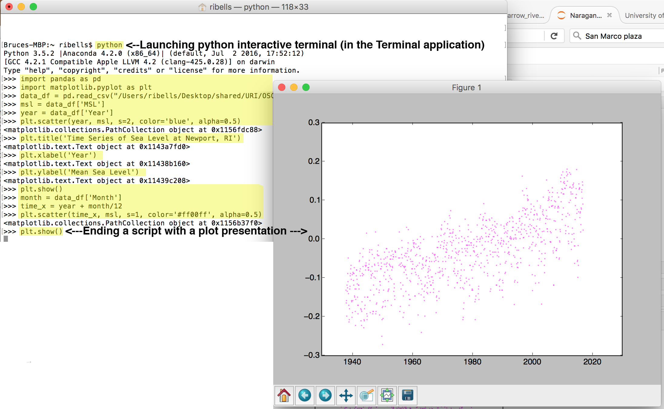

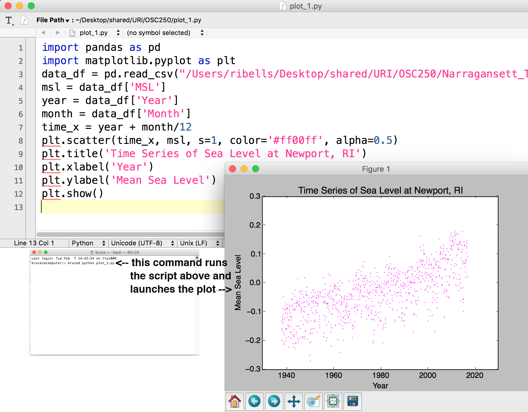
Running a Python Script from text file

Alternatively, Python commands can be batched in text files to create sequences of commands that do something useful. As an example, the figure below shows the same commands used in the interactive terminal, but as saved as lines in a text document. Python anticipates python scripts to have an .py extention. If I save these commands in a file I call plot_1.py, I can then run all of them in sequence via a single python command:

python plot_1.py

The Python interpreter can run those commands and provide me the same plot as when typing them into the interpreter one line at a time. On a very busy analysis (of water quality and quantity predictions for climate scenarios for a watershed river basin), I typically have tens or even hundreds of Python script files saved with a .py extension and a coordinated file naming scheme that helps me remember when each script is useful for analysis needs.

Automating the Week 3 Analysis

Python allows us to pass parameters into a Python script. Here's a script that allows us to do so. The script is shown below as well. Python has two libraries named sys and getopt that provide command line argument retrieval into a Python script. So, import the two libraries as seen on line 7. Lines 9-24 set up the parameter (aka argument) retrieval to assign a variable named inputfile with the csv data file name and a variable named location with the location. Lines 85 and 86 set up the conventional sys module parameter passing capability. Lines 25-83 run the script as we created it in class during week 3. The input file can now be automated on line 26. The location can now be automated on line 34.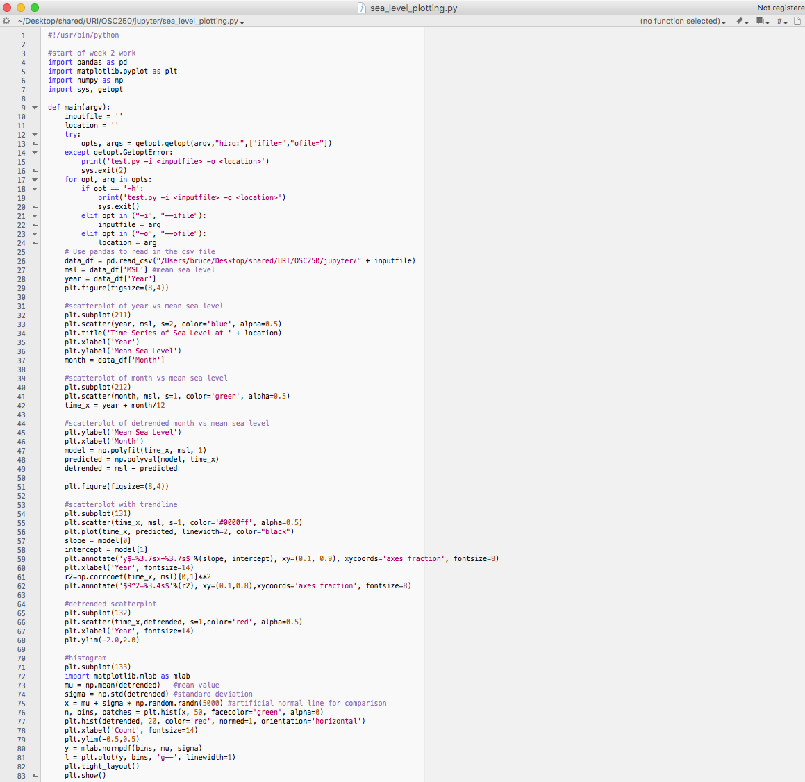


Of course, the script should be adapted to your own computer's state. You probably have saved the input files (the CSV files) in a different absolute file path on your machine (so you'll need to change the directory used in line 26). And, you may not have stripped the spaces out of the header row of your CSV files (I did so in a text editor). In that case, you'll need to add the spacing to the reference strings used on lines 27, 28, and 37.

I put the following URL (resource address) into my Web browser:

https://tidesandcurrents.noaa.gov/waterlevels.html?id=8722621&units=standard&bdate=19200213&edate=20170209&timezone=GMT&datum=MSL&interval=m&action=data

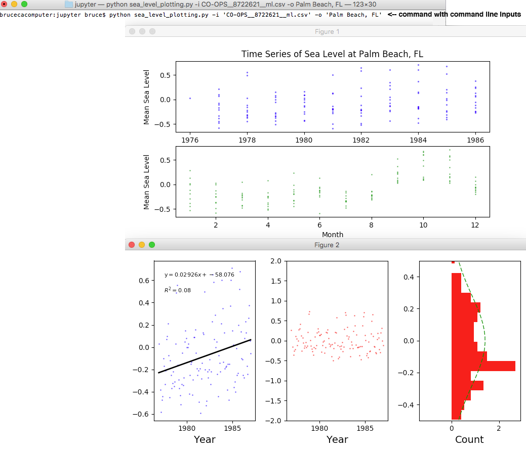
changed the units from feet to meters, and then saved the resultant data as a CSV file (using the default name CO-OPS__8722621__ml.csv). I put the file in the same directory as my Python script and ran the command:

python sea_level_plotting.py -i 'CO-OPS__8722621__ml.csv' -o 'Palm Beach, FL'

which then generated the outputs seen below:

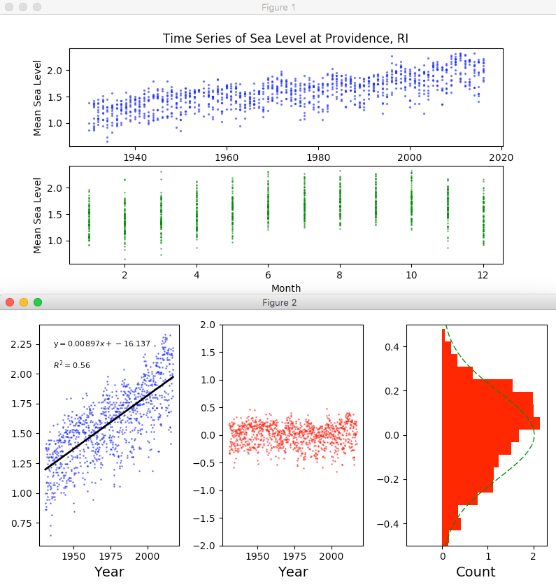
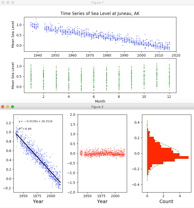
Running the Script for Providence and Juneau

I then ran the same script for the Providence and Juneau data sets we grabbed during week 1 and the script faithfully provided the results shown below: