MATLAB is another popular script-driven computing environment for doing ocean science data analysis. Below is an example of doing MATLAB work, using the classroom activity on February 8th as an example. Compare the MATLAB script with the Python script we wrote to do a similar analysis. The MATLAB script is here:

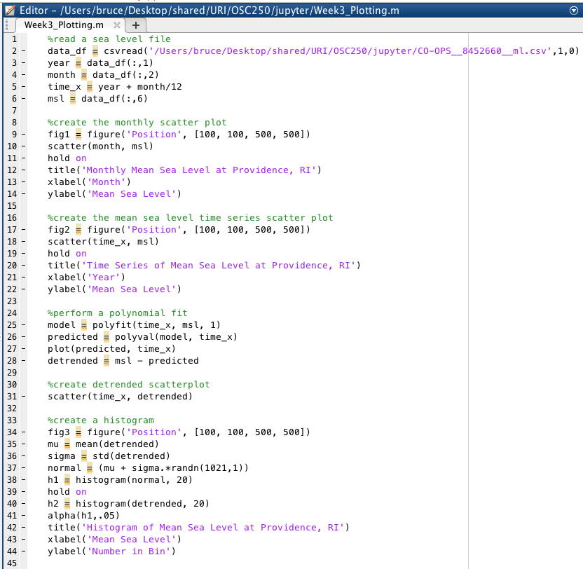
The commands are similar to the Python commands we ran but in the MATLAB case, all loaded modules are available to the script. I determine which modules load when I launch the MATLAB program. I probably have overdone it as MATLAB takes about forty seconds to load as a result of all the modules it readies at launch time. I am only using about 2% of them in the script. As I run the script within MATLAB, I can run one line at a time (like the control we have over the Jupyter notebook). After each line runs, the command window shows the result. Every variable's content is shown in its entirety after each assignment or mathematical operation (internally, MATLAB treats each variable as a matrix). For example, after I run line 25, the command window shows me:



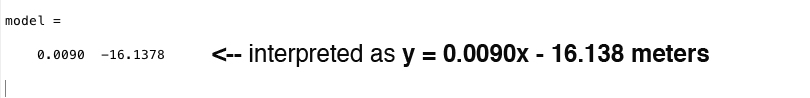
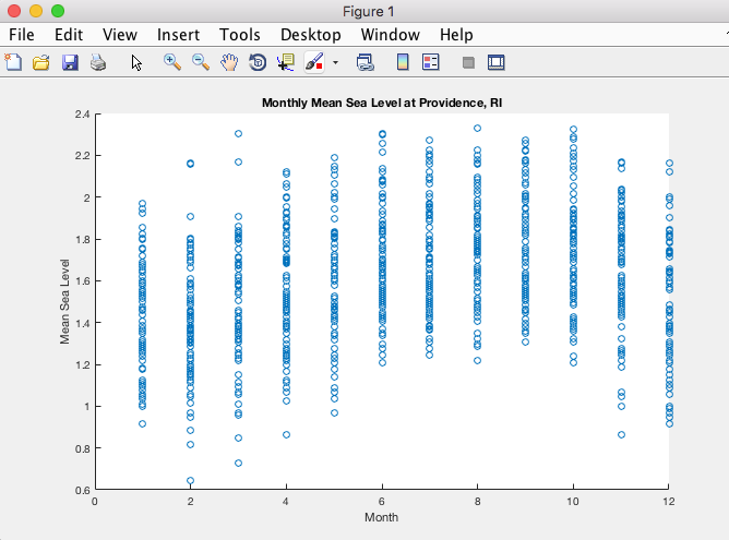
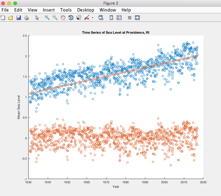
I can then take those results and generate a line from them. Running the script produces the three figures in separate application windows shown here:

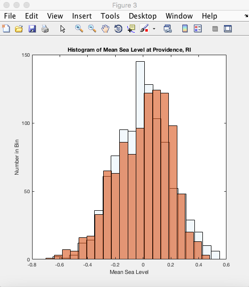
In figure 3, the white background histogram has been generated by a random fit of 1021 values using the mean and standard deviation to create them. The binning is different from the binning of the actual detrended msl data, which is shown in the faded red.