

Class on October 16 2018
Brian continued the discussion of model analysis based on the simple predator-prey models students considered last week. Brian pointed out important
things to consider for any model:
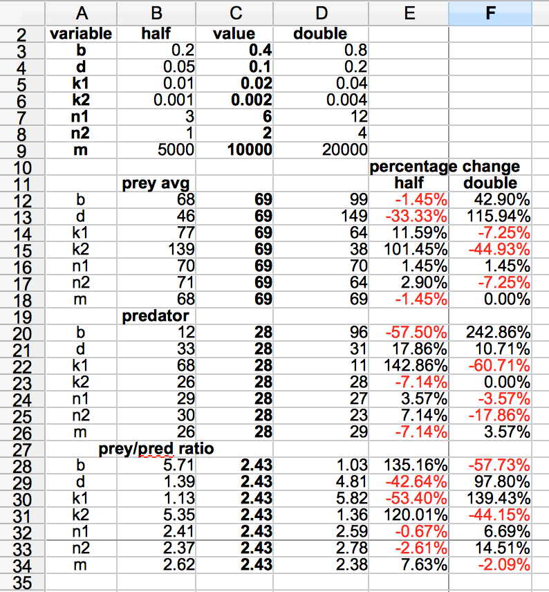
Students used the whiteboard to show their own results for predators and prey and then were asked to look for cause and effect rationale as to why the reasonability metrics changed with changes to each input variable (one at a time). Brian suggested students add variable m (the carrying capacity variable) to the list of variables they consider in their sensitivity analysis.
Jeremy made some suggestions regarding what to analyze once you think you have a good model:
- What are the units of every variable being used as inputs to the model (for time, is it seconds, minutes, hours, years, etc.? for volume is it cubic centimeters, cubic meters, etc.?). Different published works will use different units of measure so some conversions may be necessary. Older publications especially are unaware of conventions used more recently.
- Can a variable reasonably go negative? For example, Brian suggests pH can be negative and shared a story about exhaust from a space shuttle launch (his calculations showed a negative pH which NASA engineers said was impossible - is it?). What does a negative n1 or n2 mean? Can we have negative numbers of animals in a predator-prey relationship?
- Be very wary of any lines of code that mask error situations in the model. The code might have been added to make sure situations that cannot happen in the real world don't happen, but it's often best to see the the unreasonable results happen in case it spurs thoughts of other things that might be wrong in the model formulation.
- Numerical instability and strange feedback loops are worth being vigilant about when looking for situations that can suggest reasonability bounds for input variable(s) to the model.
Students used the whiteboard to show their own results for predators and prey and then were asked to look for cause and effect rationale as to why the reasonability metrics changed with changes to each input variable (one at a time). Brian suggested students add variable m (the carrying capacity variable) to the list of variables they consider in their sensitivity analysis.
Jeremy made some suggestions regarding what to analyze once you think you have a good model:
- It can be more intuitive to compute the percent change from the base level. The slope or gradient: delta(N)/delta(p) could be more useful if normalized. How would you do this? One way would be by multiplying each slope by mean(p)/mean(N).
- Look at the direction of changes — which changes were benefiting prey or predator and relate this back to the model equations.
- It is instructive to solve for the equilibria analytically by setting the rates of change to zero? How did changes in the parameters alter the steady-state prey and predator populations?
- It is interesting to see how the dynamics change when the prey carrying capacity, variable m, is increased or decreased. Are there examples from nature of increased carrying capacity?