To follow along with the example below, make sure to install the Anaconda program and explore the use of Jupyter notebooks as seen on the Jupyter Web page. In this class, we use the Python scripting language to perform data manipulation and visualization. Many people have used Python for this purpose for years. Python grew rapidly as a popular data manipulation language that processed inputs, internals, and outputs to scientific models, even allowing for models written in other languages to be wrapped by Python (see SWIG, for example) for easy data infusion and reporting purposes.

Python interprets statements one at a time where as many scientific models are written on sophisticated platforms that run code in other ways (parallel, as opposed to sequential, processing included).

Before the coordinated notebooking facilities, Python could be invoked in two popular ways (which will still work fine today on a machine where the Anaconda application suite of tools have been loaded. Below are two examples of using traditional Python means to pursue what we pursue on September 20th in class:

Running Python commands interactively in a Terminal application

Operating systems provide applications for interacting with the control of a computer through typed commands. On the Mac OS (and most flavors of Linux), there is an application called Terminal (as seen below). Within the Windows OS, there is an application called Command (or cmd or Command Prompt). Launching these programs provides access to running the python command. The python command provides an intearctive Python terminal in which code statements written in Python can be run one at a time. Below shows a terminal session whereby I typed in everything that has been highlighted in yellow (the white text are feedback output provided by the Python language). When I finish by typing the plot.show() command, a plot window appears with the identical plot that is generated when using a Jupyter Python notebook in class.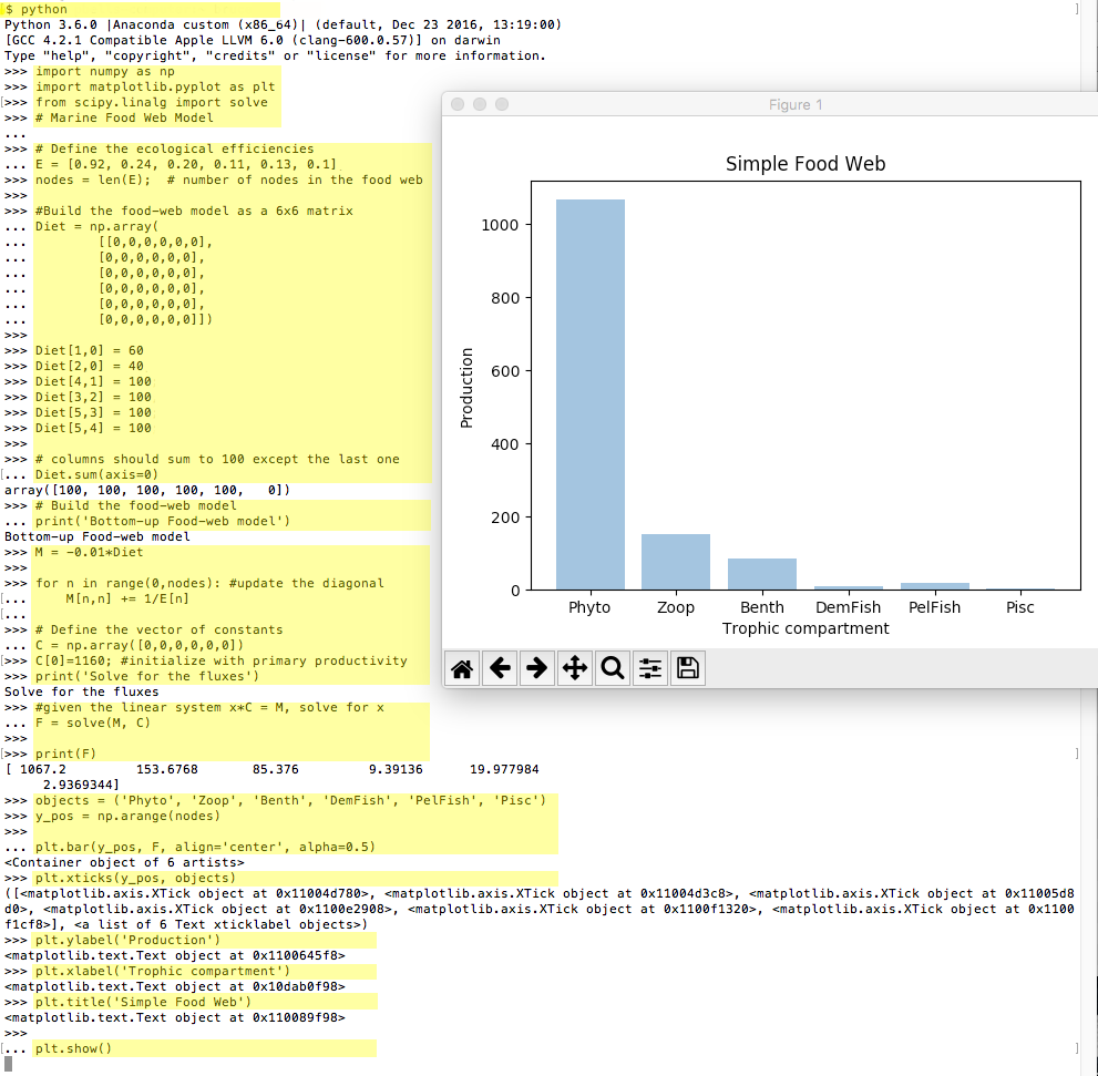

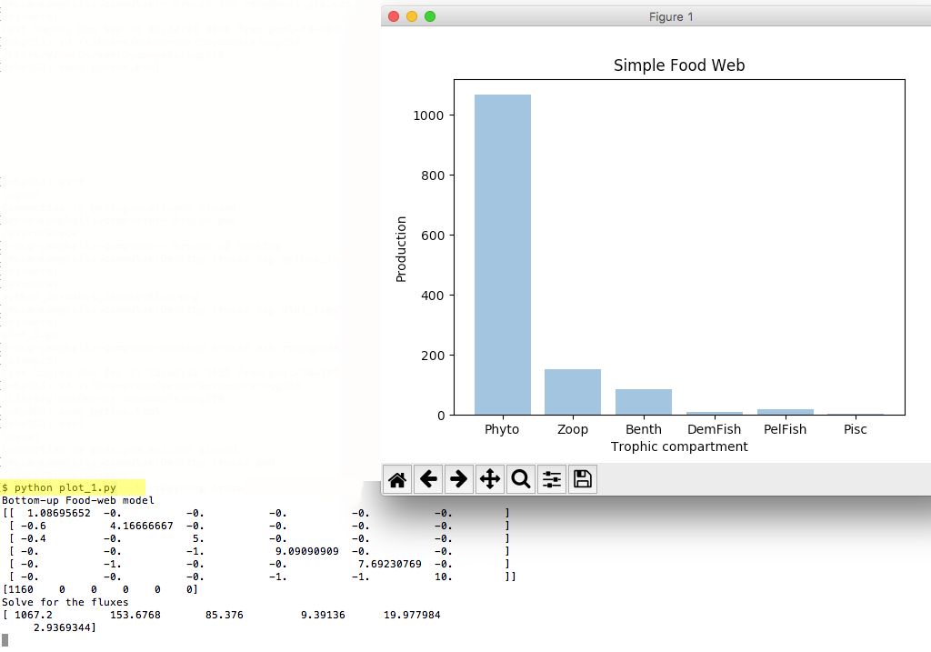
Running a Python Script from text file

Alternatively, Python commands can be batched in text files to create sequences of commands that do something useful. As an example, the figure below shows the same commands used in the interactive terminal, but as saved as lines in a text document. Python anticipates Python scripts to have an .py extention. Since I saved these commands in a file I named plot_1.py, I can then run all of them in sequence via a single python command:

python plot_1.py

The Python interpreter can run those commands and provide me the same plot as when typing them into the interpreter one line at a time. On a very busy analysis (of water quality and quantity predictions for climate scenarios for a watershed river basin), I typically have tens or even hundreds of Python script files saved with a .py extension and a coordinated file naming scheme that helps me remember when each script is useful for analysis needs.

Using Jupyter Notebook

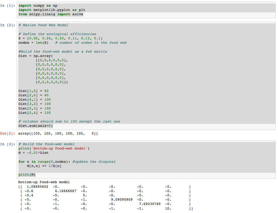
The Jupyter Python notebook service affords piecemeal development and running of Python code. Python services can be imported via the import ... as or from import statements that are included in the base Python language. This first example uses three very popular Python packages to do useful work in a notebook: NumPy, MatPlotLib, and SciPy. NumPy is the fundamental package for scientific computing with the Python language. Matplotlib is a Python 2D plotting library which produces publication quality figures in a variety of hardcopy formats and interactive environments across platforms. SciPy is a Python-based ecosystem of open-source software for mathematics, science, and engineering. As SciPy contains many sub-packages, it is common to ask for just one of the packages as in the scipy.linalg example seen in section [1] of the notebook screenshot below (linalg is a linear algebra sub-package used for solving sets of linear equations that have certain properties).

The base Python language provides a useful print() function to print the value of any intermediate variable involved in a computation or visualization. Section [3] of the partial notebook screenshot below demonstrates the use of the print() function to print the state of a variable named M, which is being managed as a matrix.

In this class, learning Python requires learning the rules of syntax for writing valid code, learning how to declare variables and initialize them with data, learning how to perform useful computation and visualization with those data, and learning which approaches provided by which packages are the best for an overall data analysis activity.

In section [2] of the notebook screenshot below, a variable named E is declared as containing a collection of six numbers, each an ecological efficiency ratio for an organism relationship in a food web. The use of [ and ] symbols is a very common convention for creating a collection. Values in the collection can be referred to by offset. For example, E[0] refers to the first value of 0.92, while E[3] refers to the fourth value of 0.11 (offset by 3 from the first). The variable nodes is being declared to hold a single whole number (integer) of 6, the length of the E collection.

In section [2] another collection, named Diet, is being set up through NumPy's array() constructor, which allows for two-dimensional stores of data. Although the collection is being created as a 6x6 array of 0s, it is then being updated to store other values through updating one value at a time. In section [3] the line Diet[1,0] = 60 updates the first value of the second row from 0 to 60 (offsets start with 0 no matter how many dimensions are being stored). The line M = -0.01*Diet multiplies each of the 36 values of the Diet collection by -0.01 and declares a collection named M which Python initializes as a 2-D collection with the same size as the Diet collection.

Section [3] also contains a for loop. A for loop lets one or more lines of code run multiple times (in this case nodes, or 6, times) by using a new variable (in this case n) to perform work (setting the diagonal values in the 6x6 collection that will be used as a matrix typical of many food web calculations). Take a close look at the screenshot below to get a sense of the flow of Python. The lines that begin with a hashtag (#) symbol are just comments for code documentation. They are not run by the notebook. Code that is indented with the tab character is treated as a block (when associated with a for loop, for example). The screenshot ends with result of printing the M variable for inspection.



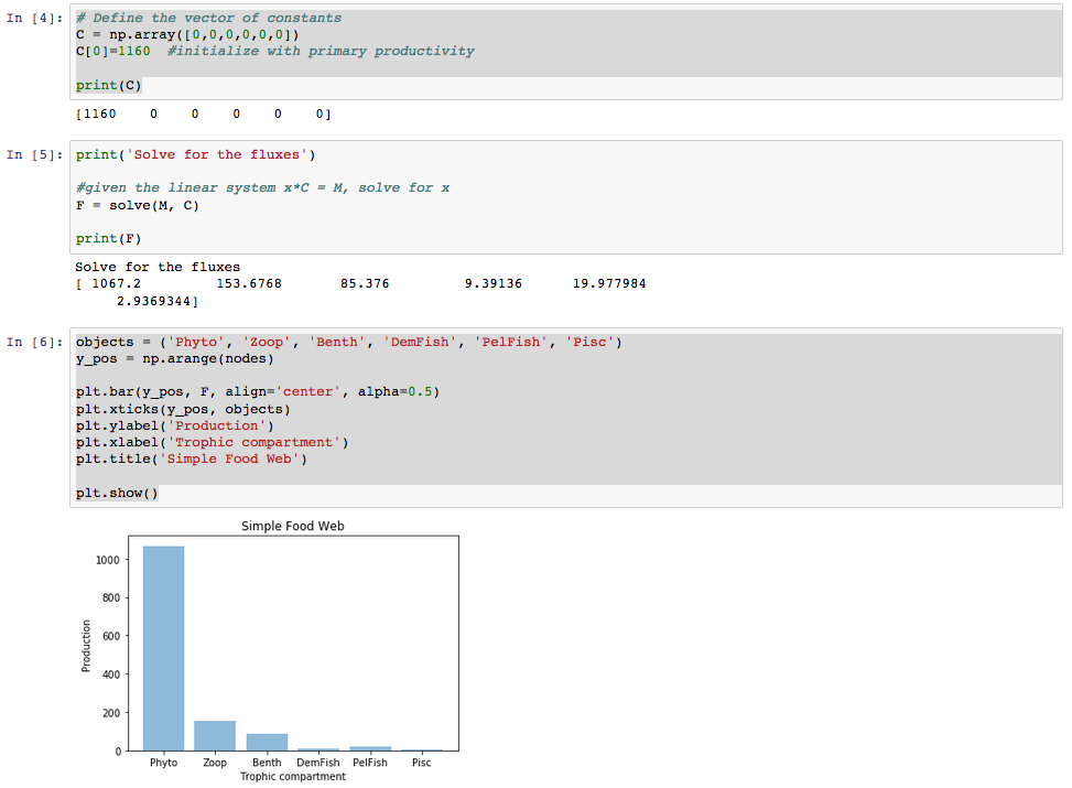
The next section of a Jupyter Python notebook is shown below. Section [4] creates another 1-dimensional collection and sets the first value to 1160 before printing it for verification. Section [5] uses the solve() service from the linear algebra sub-package to solve for food web fluxes (and stores the results in a new collection named F). Section [6] creates a 1-dimensional text-based collection (using parentheses creates a list format), creates a range of values from 0 to 5 (nodes number of them), and then uses the Matplotlib services to create the bar chart seen as a result of the plt.show() statement (remember that the plt refers to the imported matplotlib.pyplot services requested in section [1] of the notebook (just as the services prefixed by np. were provided by numpy, and prefixed by solve. were provided by scipy.linalg as imported in section [1)].



Python syntax varies slightly depending on the programmer who scripted the services in each available package, but the base Python language syntax aims to be consistent as managed by a Python language committee. Python is generally considered to have become so popular because of the writability and consistency provided over many years.

Try and gain an instinct to how Python code is written so you can rely on that instinct to remove clutter from those things you have to memorize or refer to often in reference documents online. If you organize all the code you write or study into a library of code, you'll be able to reuse syntax structures for similar analysis tasks.