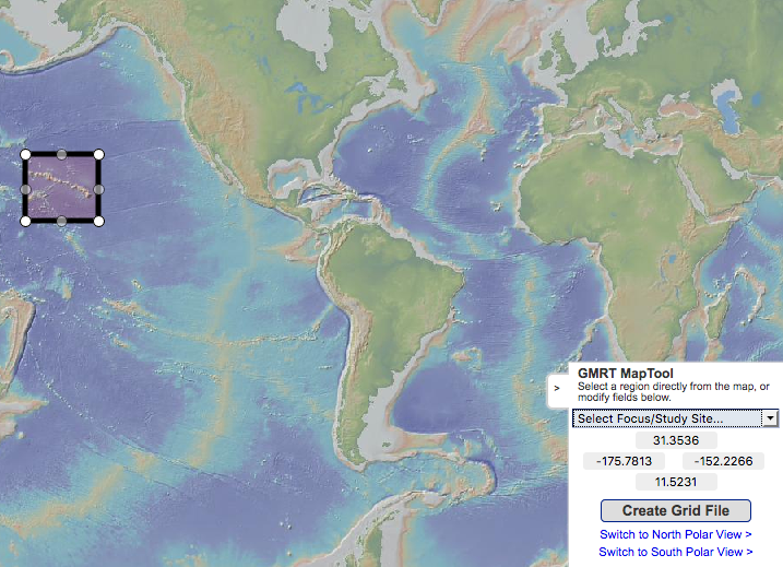
Rob spent the class introducing NetCDF grids to complement the sandbox exercise with the use of global terrain data. Global terrain is available at the GMRT Map Tool online. As seen in the image below, the site allows a user to create a rectangle around a geographical area of interest (the Hawaiian islands in this case). The study site bounds in latitude and longitude are then reported in the lower left of the tool.



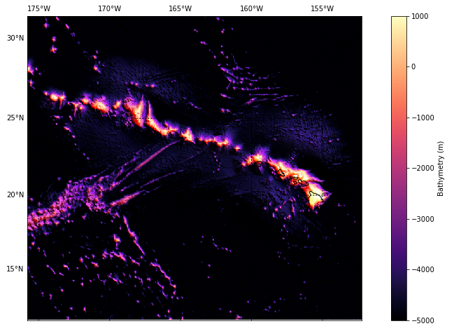
Rob provided a starter Jupyter Python notebook for NetCDF grid plotting. The download format from the GMRT Map tool is NetCDF by default. We use the latitude bounds of [11.5321, 31.3536] and longitude bounds of [-175.7813,-152.2266] as parameters to the Basemap generation process. We played with color map choices using the related Matplotlib documentation. Using the magma color map provides the plot image seen here:



Other decisions typically made by scientists during analysis include:

• projection (e.g. 'merc' for mercator)
• resolution (crude, low, intermediate, high, full)
• illumination angle (to provide dramatic shading)
• vertical exaggeration (to facilitate visual analysis)
• coastlines and political borders (to facilitate recognition)

Students were asked to continue to work with the notebook to play with the area coverage they downloaded as well with two grid files Rob provided:

• age.3.6.grd
• chl.grd

The variables property of each loaded NetCDF file reports on the variable names, types, and dimensions. So, for the age.3.6.grd file, bathymetry, longitude, and latitude have variable names of z, x, and y respectively and the assignment step becomes:

bathy = fh.variables['z'][:]
lons = fh.variables['x'][:]
lats = fh.variables['y'][:]

There is a lot to learn about human perception and cognition through investigating all the options.