

Class on March 20 2018
Rob provided an overview of filtering techniques for performing an analysis of water level. Sampling rates were every six weeks, a much higher
sampling rate than the mean water level values calculated for a monthly temporal resolution that were used the previous week. To demonstrate the
effect of combining multiple samples into means, Rob had students use their spreadsheet tool to create the chart demonstrated here:
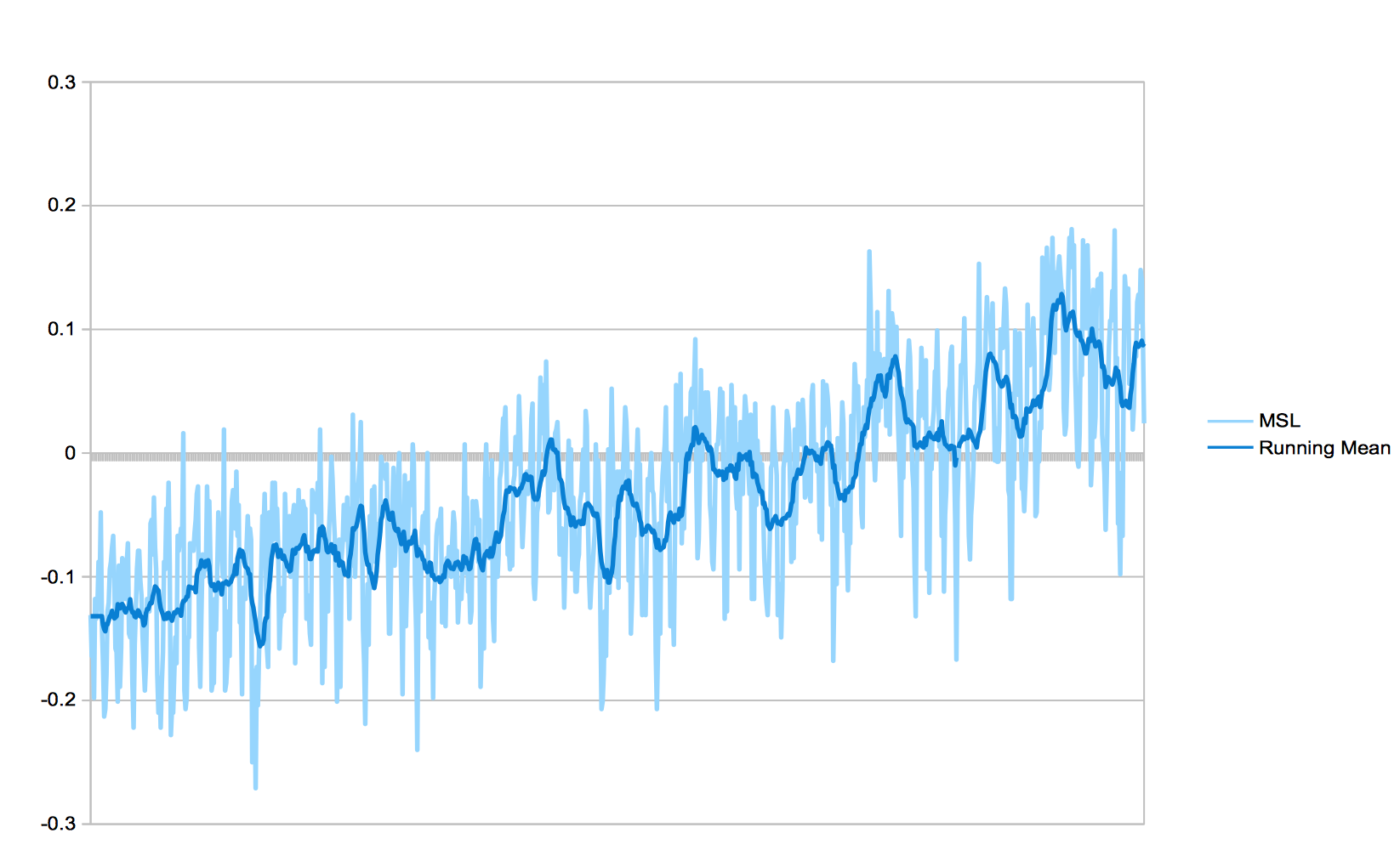
The general long-term pattern is easier to see via a plot of monthly means than the monthly values. Filtering techniques are techniques to look at a complex data set in search of patterns. A low-pass filter removes any short wavelength waves out of data. A high-pass filter removes the long wavelength waves out of data. In the case of a pond temperature data set (with two sensors at surface and depth), a low-pass filter can remove any noise provided by the limits of physical hardware. A high-pass filter can specifically look at the amount of potential noise in the data.
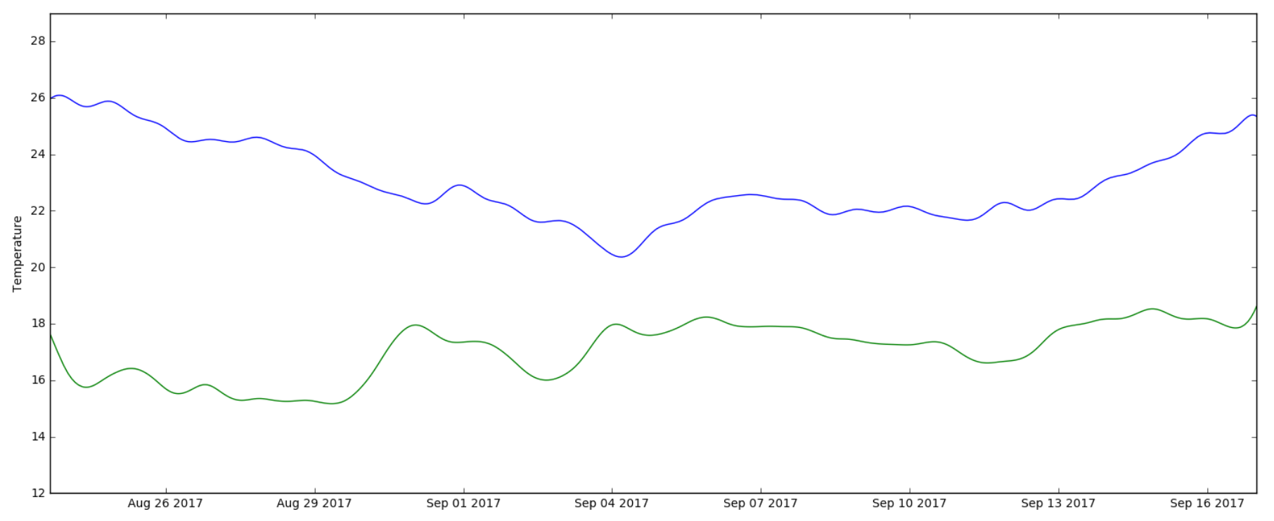
Filters can be applied to spatial data as well as the temporal data students considered in class. Rob demonstrated a low-pass filter that removed noise and tidal data out of a pond temperature dataset. Using Python, a low-pass fiter can be applied to the surface temperature data via:
Plotting the results of the low-pass filter created the image:
Students then changed the bounds of the filter to create a high-pass filter to focus in on the noise inherent in the two location signals:
Plotting the results of the high-pass filter created the image:
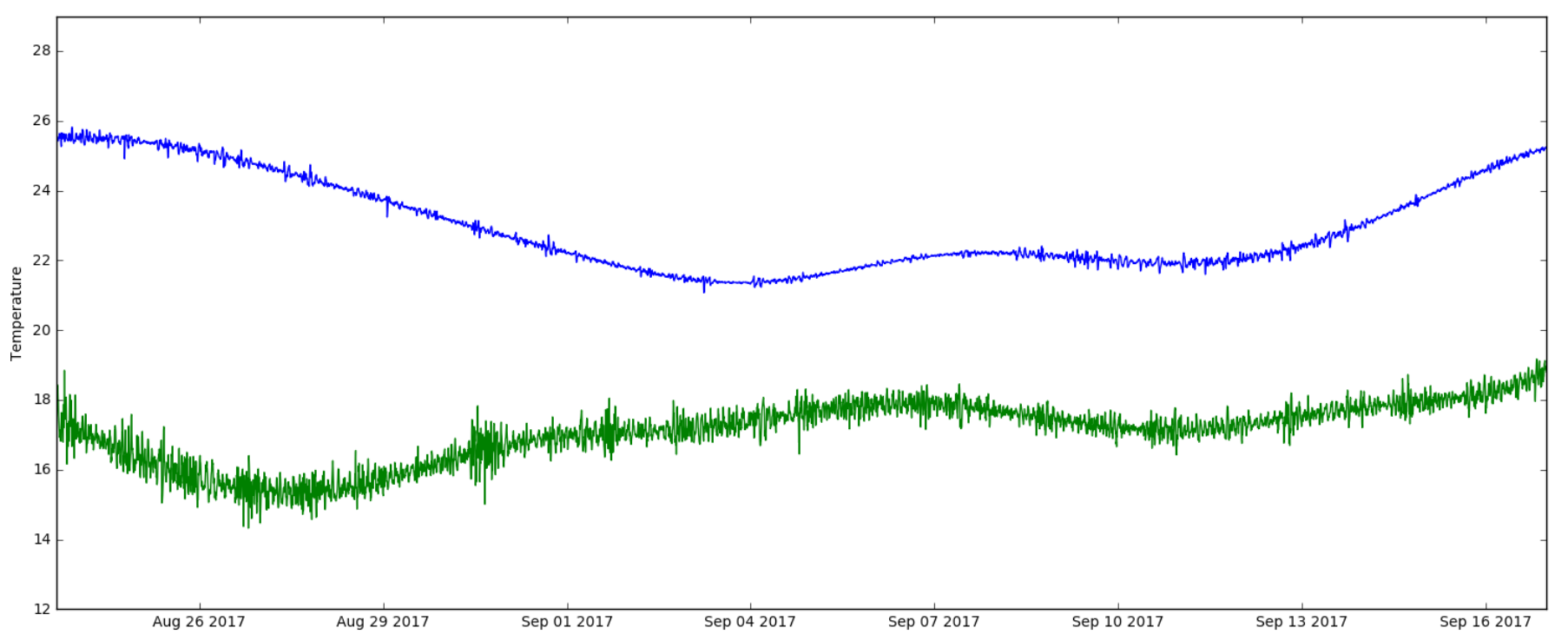
The analysis suggests that the deeper sensor was more noisy than the upper sensor. Since usually there is more variability at the surface (since air temperature and wind have a higher effect there), the results are curious and suggest that perhaps the sensor at depth is less reliable in its ability to sense temperature (or else some rare process was changing temperature more dramatically at depth).
Students were asked to consider other filters that might be of interest when looking at the sensor data set. They were asked to organize plots into one analysis using plot layout techniques studied in previous classes.
The general long-term pattern is easier to see via a plot of monthly means than the monthly values. Filtering techniques are techniques to look at a complex data set in search of patterns. A low-pass filter removes any short wavelength waves out of data. A high-pass filter removes the long wavelength waves out of data. In the case of a pond temperature data set (with two sensors at surface and depth), a low-pass filter can remove any noise provided by the limits of physical hardware. A high-pass filter can specifically look at the amount of potential noise in the data.
Filters can be applied to spatial data as well as the temporal data students considered in class. Rob demonstrated a low-pass filter that removed noise and tidal data out of a pond temperature dataset. Using Python, a low-pass fiter can be applied to the surface temperature data via:
def butter_bandpass(lowcut, highcut, fs, order=1):
    nyq = 0.5 * fs
    low = lowcut / nyq
    high = highcut / nyq
    b, a = butter(order, [low, high], btype='band')
    return b, a

def butter_bandpass_filter(data, lowcut, highcut, fs, order=1):
    b, a = butter_bandpass(lowcut, highcut, fs, order=order)
    y = signal.filtfilt(b, a, data)
    return y

fs = 10         #samples per hour (10 at 6min intervals)

#   ----------  synoptic
fine = 0.20001  #lowest frequency (Nyquist) is 2x sampling rate (1/fs or 0.1)
tidal = 33      #cutoff to remove tidal signals (33 hours is three tidal cycles)

#   ----------  frequency
lowcut = 1/tidal
highcut = 1/fine

S_t1 = butter_bandpass_filter(surface_temp, lowcut, highcut, fs, order=3)
S_rsd_t1 = surface_temp - S_t1

S_t2 = butter_bandpass_filter(depth_temp, lowcut, highcut, fs, order=3)
S_rsd_t2 = depth_temp - S_t2
Plotting the results of the low-pass filter created the image:
Students then changed the bounds of the filter to create a high-pass filter to focus in on the noise inherent in the two location signals:
S_t3 = butter_bandpass_filter(surface_temp, (1/176), (1/3), fs, order=3)
S_rsd_t3 = surface_temp - S_t3

S_t5 = butter_bandpass_filter(depth_temp, (1/176), (1/3), fs, order=3)
S_rsd_t5 = depth_temp - S_t5
Plotting the results of the high-pass filter created the image:
The analysis suggests that the deeper sensor was more noisy than the upper sensor. Since usually there is more variability at the surface (since air temperature and wind have a higher effect there), the results are curious and suggest that perhaps the sensor at depth is less reliable in its ability to sense temperature (or else some rare process was changing temperature more dramatically at depth).
Students were asked to consider other filters that might be of interest when looking at the sensor data set. They were asked to organize plots into one analysis using plot layout techniques studied in previous classes.