

Class on February 11 2019
Chris reminded students to keep working on the homework assignment 3 through the weekend.
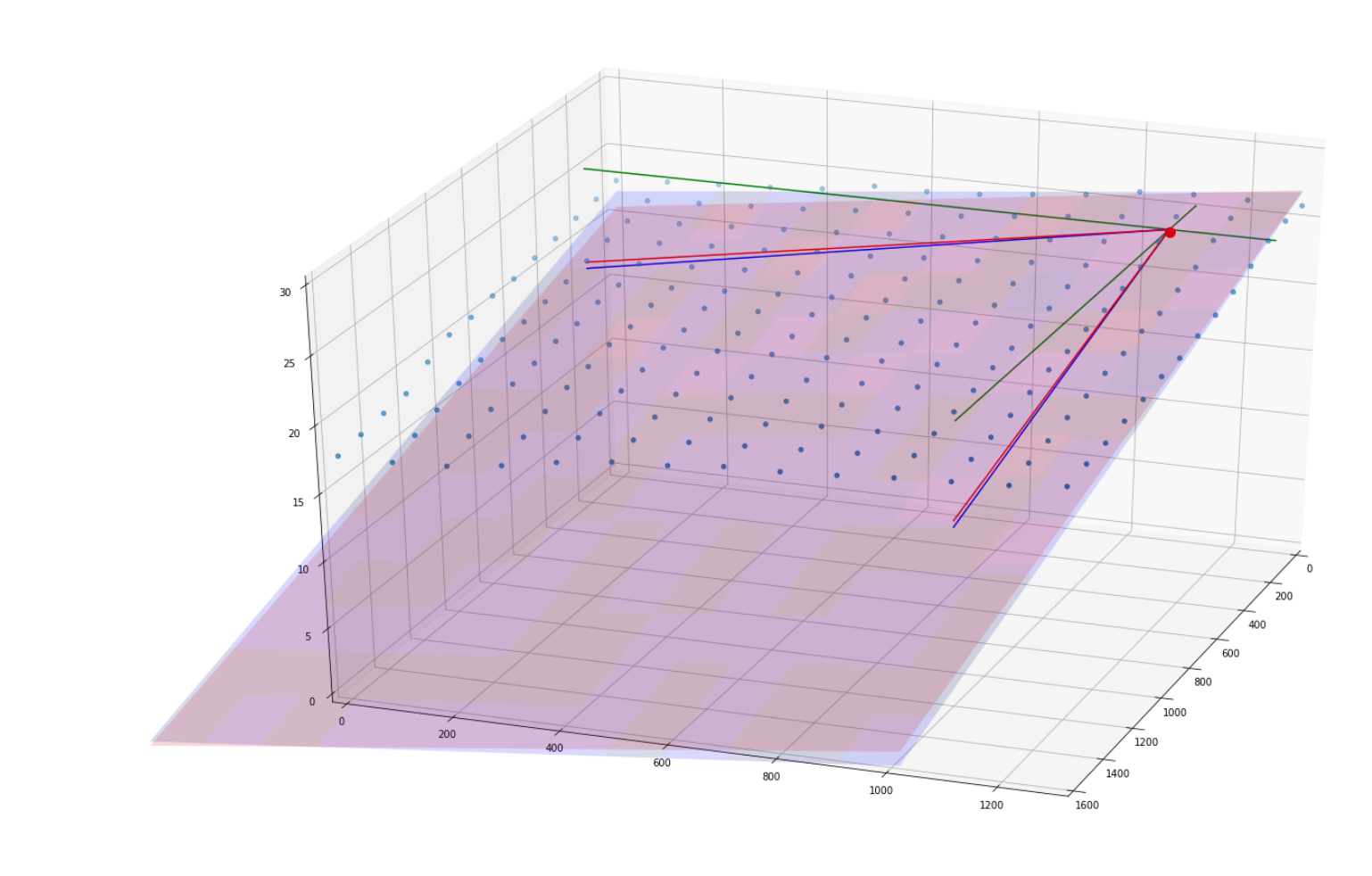
A Python notebook equivalent is available for considering plotting techniques:
Chris introduced the watt as a unit of measure, calculated as Joules per second (W = J/S). Heat Flux is described in terms of watts/m2.
Chris provided a review of the work we had done on heat flow in the previous class:
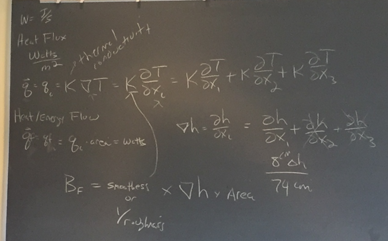
Although we only looked at the change in height in one direction (x1), there are three directions for potential change (hence our vector axes). K is the thermal conductivity variable.
Chris then expanded upon the conservation of energy as an equation we would be working with often:
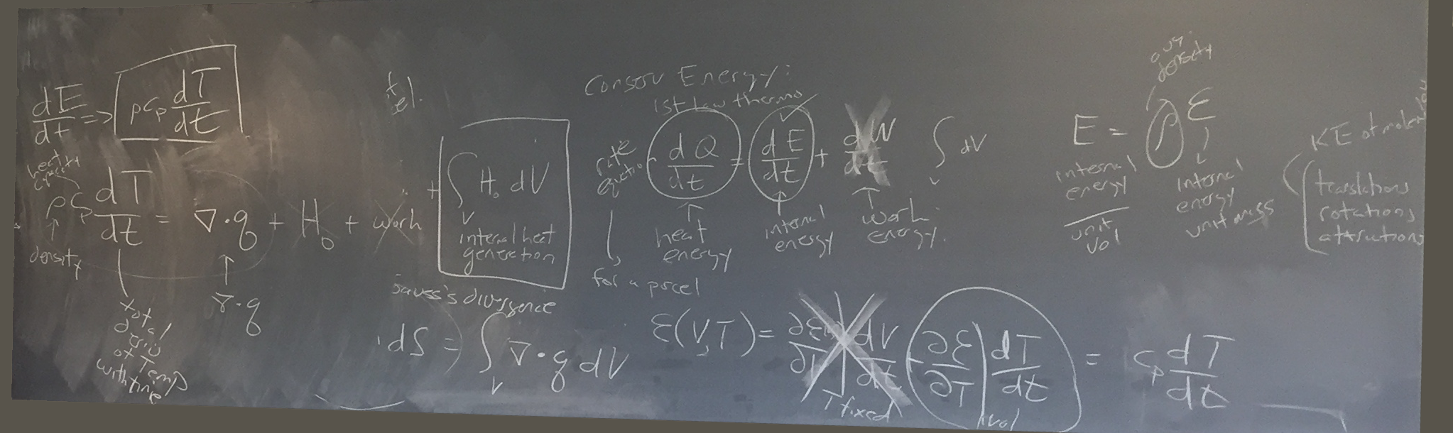
Chris suggested heat energy = internal energy + work energy (to be worked on later), whereby internal energy/unit volume = ρ * ε
ρ is average density
ε is internal energy per unit mass
There is a relationship between the temperature and the amount of energy.
For example: A British Thermal Unit (BTU) is the amount of energy required to raise temperature one degree Kinetic energy includes translations, rotations, and attractions of molecules within the fluid
We looked at energy as a function of volume and time Energy(volume, time).
dE/dt (the change in energy) = ρ * cp * dT/dt
cp is the heat capacity (in unite of Joules/kg/degree)
We can integrate dQ/dt * dV over the x1, x2, x3 (to get the total heat over all parcels)
but we can break that down into two pieces:
1. integrate the six bounding surfaces over q . ñ * dS
2. integrate the volume over H0 * dV
q is the heat flux
ñ is the normal vector (with a length of 1 normal to the surface)
Chris provided a visual explanation of how the ñ vector is determined (get the normal perpendicular to the surface at a magnitude based on the dot product — the shadow cast from the directional flow vector).
The surface integration is the harder of the two mathematically, but can be calculated using Gauss' divergence:
integrate over ▽ . q * dV
ρ * cp * dT/dt = ▽ . q + H0 + work
which is: density * heat capacity * total derivative of temperature with time
Chris provided another exercise to gain insight into the energy equation — three parcels with a focus on the intermediary one (bead bin):
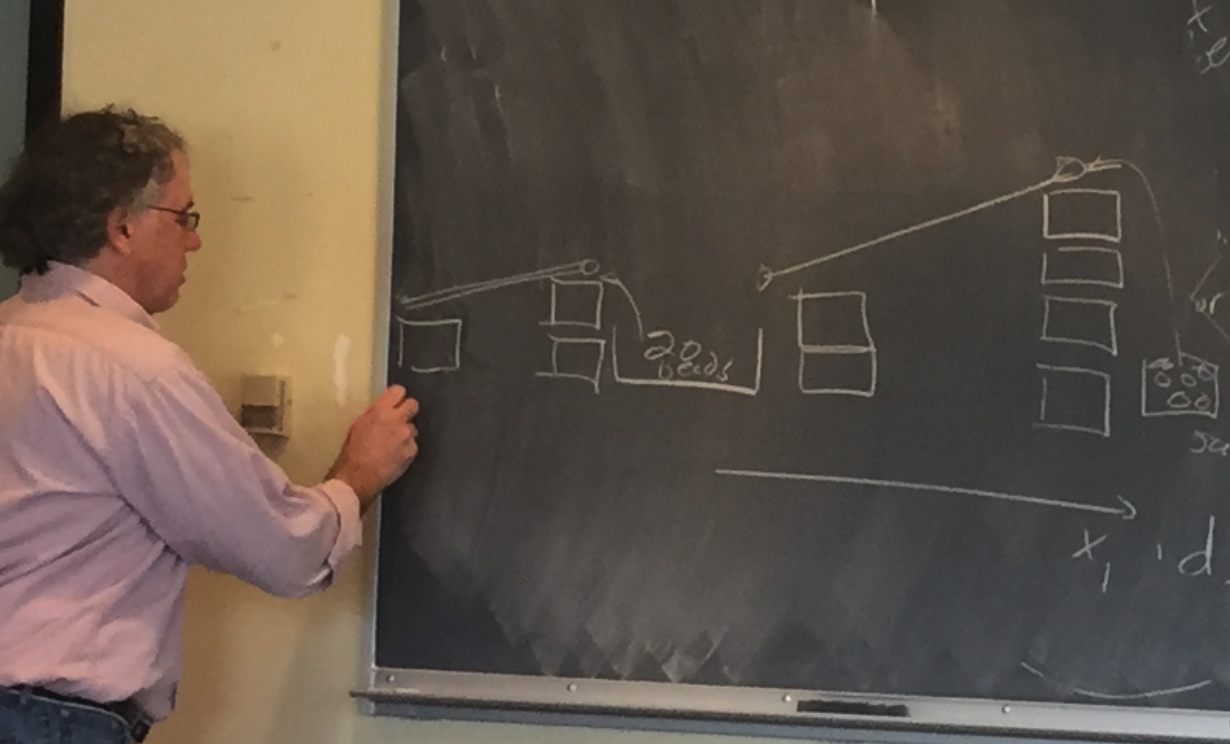
Students set up their experiments in teams to look like:
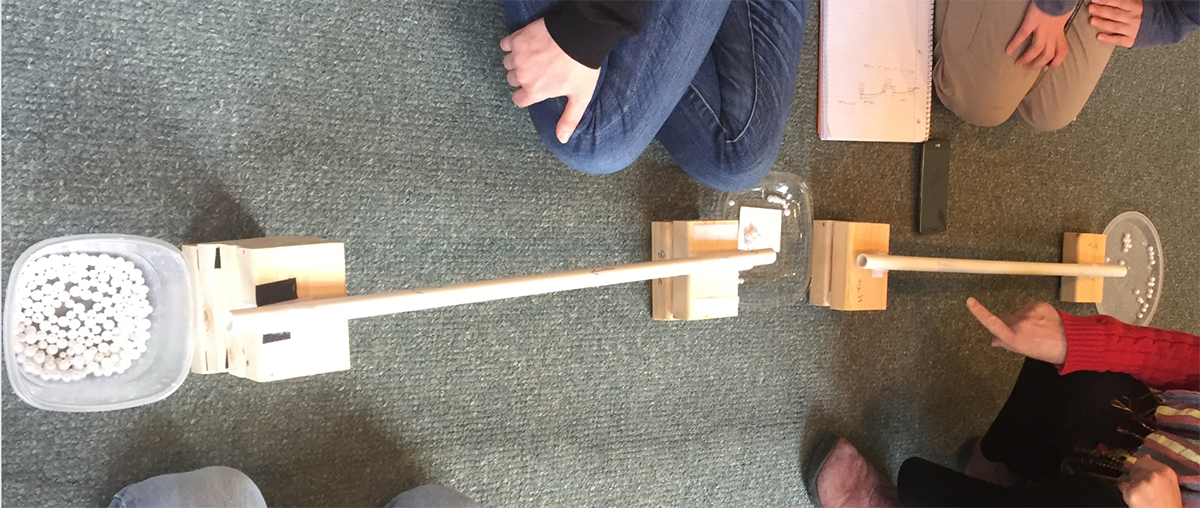
using a configuration of blocks, tubes, and balls. The middle bin is accumulating balls because the slope in is higher than the slope out,
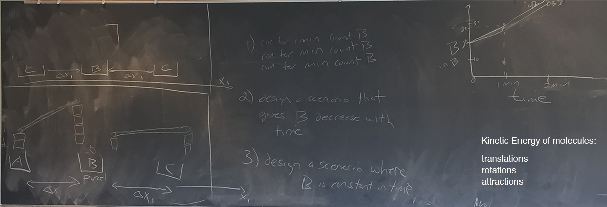
Chris asked student teams to provide configurations (seen on the blackboard above) that decreased the ball count in the middle bin and then as a class to create a bin with pipes connecting in four directions (to consider a 2-D heat transfer simulation).
Of course, heat can transfer in three directions which was left as a thought exercise.
Chris introduced the watt as a unit of measure, calculated as Joules per second (W = J/S). Heat Flux is described in terms of watts/m2.
Chris provided a review of the work we had done on heat flow in the previous class:
Although we only looked at the change in height in one direction (x1), there are three directions for potential change (hence our vector axes). K is the thermal conductivity variable.
Chris then expanded upon the conservation of energy as an equation we would be working with often:
Chris suggested heat energy = internal energy + work energy (to be worked on later), whereby internal energy/unit volume = ρ * ε
ρ is average density
ε is internal energy per unit mass
There is a relationship between the temperature and the amount of energy.
For example: A British Thermal Unit (BTU) is the amount of energy required to raise temperature one degree Kinetic energy includes translations, rotations, and attractions of molecules within the fluid
We looked at energy as a function of volume and time Energy(volume, time).
dE/dt (the change in energy) = ρ * cp * dT/dt
cp is the heat capacity (in unite of Joules/kg/degree)
We can integrate dQ/dt * dV over the x1, x2, x3 (to get the total heat over all parcels)
but we can break that down into two pieces:
1. integrate the six bounding surfaces over q . ñ * dS
2. integrate the volume over H0 * dV
q is the heat flux
ñ is the normal vector (with a length of 1 normal to the surface)
Chris provided a visual explanation of how the ñ vector is determined (get the normal perpendicular to the surface at a magnitude based on the dot product — the shadow cast from the directional flow vector).
The surface integration is the harder of the two mathematically, but can be calculated using Gauss' divergence:
integrate over ▽ . q * dV
ρ * cp * dT/dt = ▽ . q + H0 + work
which is: density * heat capacity * total derivative of temperature with time
Chris provided another exercise to gain insight into the energy equation — three parcels with a focus on the intermediary one (bead bin):
Students set up their experiments in teams to look like:
using a configuration of blocks, tubes, and balls. The middle bin is accumulating balls because the slope in is higher than the slope out,
Chris asked student teams to provide configurations (seen on the blackboard above) that decreased the ball count in the middle bin and then as a class to create a bin with pipes connecting in four directions (to consider a 2-D heat transfer simulation).
Of course, heat can transfer in three directions which was left as a thought exercise.