

Class on February 4 2019
Chris started the class with a discussion on the second homework assignment after a quick mention of terms from geology:
The dip is the acute angle that a rock surface makes from a horizontal plane. The strike is the direction of the line formed by the intersection of a rock surface with a horizontal plane. Strike and dip, as vectors, are always perpendicular to each other.
Students discussed ways to present answers to the homework questions. Some helpful Python approaches are available in this plotting approaches code that can be run with Jupyter notebook software (right mouse-click and choose Save Link As to maintain the notebook syntax).
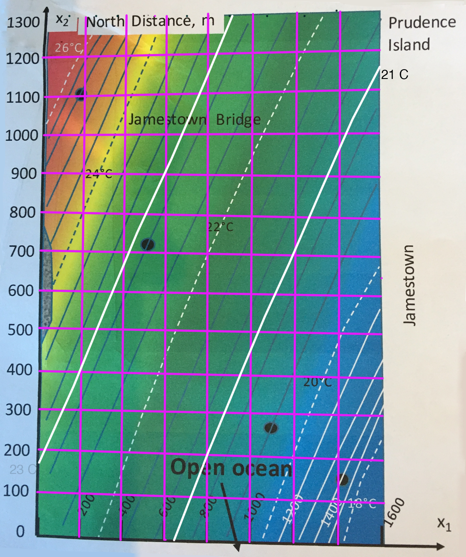
The notebook recreates the data in a 3-D plot through the use of a grid from the homework 2-D plot. The grid represents data points read from the contours and placed into a 14 x 14 array:
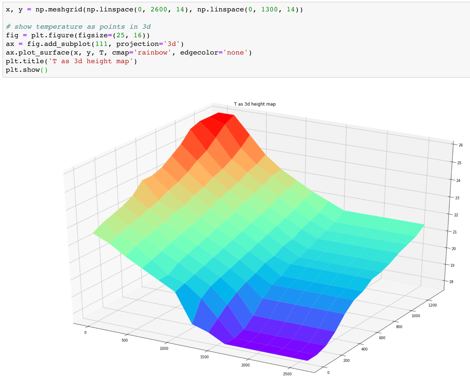
which can then be plotted as a surface:
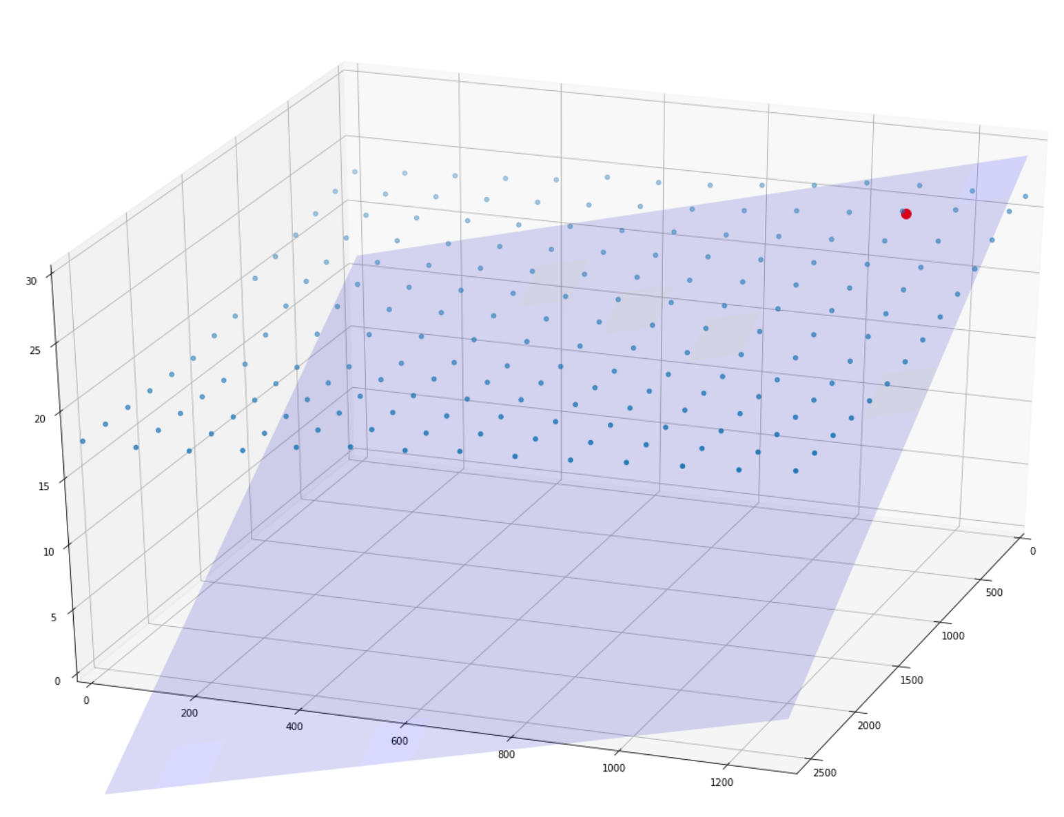
Chris asked students about the significance of the two slopes needed to get the tangential plane at a station's data (for example, the station in the upper left):
The station is at point: [190, 1105, 25.2]
data point from incremental in x1 (east from there): [200, 1105, 25.1]
data from incremental in x2 (south from there): [190, 1095, 25.1]
Three points define a unique plane (as do two vectors such as the vector from station to incremental x1 point and station to incremental x2 point as seen in the previous class).
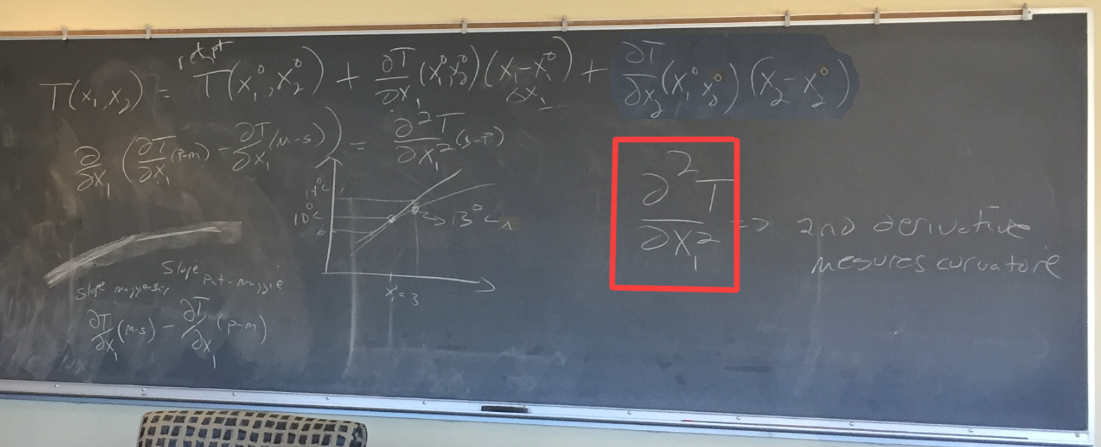
The tangential plane is just the combination of two lines, whereas a single line is formulated as seen in the blackboard here (under the familiar tangential plane formula):
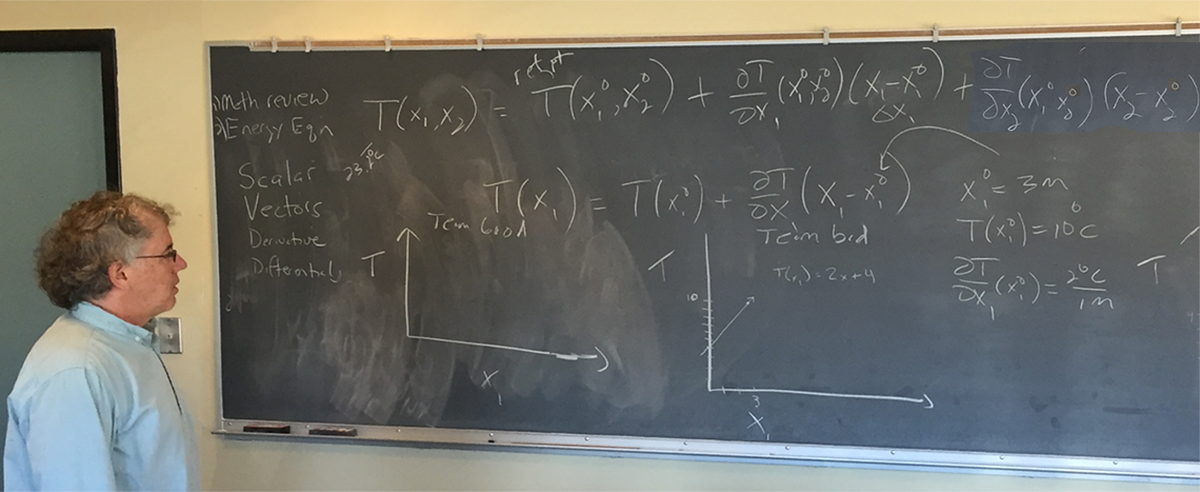
The students did an example of plotting a line with requirements x10 = 3 meters, T(x10) = 10 degrees Celsius, and delta slope is 2 degrees Celsius per meter. Three teams plotted the line through x10 (one team seen on the blackboard above.
Chris then asked students to think about three contiguous points in x1. Those points provide two transitionary vectors:

The curvature through a point transitioning between the two vectors is best described by the 2nd derivative, as seen within the red box here:
Rob suggested a useful reminder is that velocity is a first derivative and acceleration is a second derivative.
Chris then began a discussion on differentials, introducing the del operator (symbolized by ▽) as a vector seen in the red box here:

The del operator is typically used in matrix multiplications such as with the vector to the right of the red box. Expansions of del operator use include the example with T as temperature, seen in the lower right of the blackboard image above. The yellow bordered formula is the tangential plane, with the green bordered component the scalar reference point. The light blue bordered term components are the delta slopes in the x1 and x2 directions, each multiplied by a coefficient scalar of the delta distance in those directions.
Chris had student teams expand three dot products, one between vectors A and B, one between u~ and ▽ T, and one between ▽ and q~ (the heat flux), suggesting these expansions will be done often in class so students should get a lot of practice doing them on paper by hand. The course will grow to a creshendo where canceling out terms on the blackboard will become a powerful mathematical action.
Students were asked to finish homework set 2 for next class.
The dip is the acute angle that a rock surface makes from a horizontal plane. The strike is the direction of the line formed by the intersection of a rock surface with a horizontal plane. Strike and dip, as vectors, are always perpendicular to each other.
Students discussed ways to present answers to the homework questions. Some helpful Python approaches are available in this plotting approaches code that can be run with Jupyter notebook software (right mouse-click and choose Save Link As to maintain the notebook syntax).
The notebook recreates the data in a 3-D plot through the use of a grid from the homework 2-D plot. The grid represents data points read from the contours and placed into a 14 x 14 array:
import numpy as np
import matplotlib.pyplot as plt
from mpl_toolkits.mplot3d import Axes3D
import math as math

T = np.array([
    [22.6,22.2,21.6,21.1,20.6,20.1,18.4,18.1,17.6,17.6,17.6,17.6,17.6,17.6],
    [22.9,22.4,21.9,21.3,20.6,20.3,19.6,18.6,17.6,17.6,17.6,17.6,17.6,17.6],
    [23.1,22.6,22.1,21.5,21,20.5,20,19.1,17.8,17.8,17.8,17.8,17.8,17.8],
    [23.3,22.8,22.3,21.7,21.2,20.7,20.2,19.5,18.3,18.3,18.3,18.3,18.3,18.3],
    [23.6,23,22.4,21.9,21.4,20.9,20.4,19.8,19,19,19,19,19,19],
    [24.2,23.2,22.7,22.1,21.6,21.1,20.6,20,19.5,19.5,19.5,19.5,19.5,19.5],
    [24.2,23.5,22.8,22.3,21.8,21.3,20.8,20.3,19.7,19.7,19.7,19.7,19.7,19.7],
    [24.4,23.7,23.1,22.5,22,21.5,21,20.4,20.1,20.1,20.1,20.1,20.1,20.1],
    [24.8,24,23.3,22.8,22.2,21.7,21.2,20.7,20.2,20.2,20.2,20.2,20.2,20.2],
    [25.2,24.4,23.6,23,22.5,21.9,21.4,20.8,20.4,20.4,20.4,20.4,20.4,20.4],
    [25.8,24.7,23.8,23.2,22.7,22.1,21.6,21.1,20.7,20.7,20.7,20.7,20.7,20.7],
    [26,25.2,24.1,23.5,22.9,22.4,21.8,21.3,20.9,20.9,20.9,20.9,20.9,20.9],
    [26,25.7,24.5,23.7,23.2,22.6,22.1,21.5,21.1,21.1,21.1,21.1,21.1,21.1],
    [26,26,25,24,23.3,22.8,22.3,21.9,21.5,21.5,21.5,21.5,21.5,21.5]
],object)
which can then be plotted as a surface:
#add a station point and draw the tangential plane from three points
#(or as two vectors)
p1 = np.array([190, 1105, 25.2])
p2 = np.array([200, 1105, 25.1]) #data from incremental in x1
p3 = np.array([190, 1095, 25.1]) #data from incremental in x2

# These two vectors are in the plane
v1 = p3 - p1
v2 = p2 - p1

# the cross product is a vector normal to the plane
normal = np.cross(v1, v2)
a, b, c = normal

# formula for a plane is a*x+b*y+c*z+d=0
# [a,b,c] is the normal.

# so we have to calculate d from the station point
d = -p1.dot(normal)

# create an x,y mesh for uniform points on the plane
xx, yy = np.meshgrid(np.linspace(0, 2600, 14), np.linspace(0, 1300, 14))

# calculate each corresponding z on plane
z = (-normal[0] * xx - normal[1] * yy - d) * 1. /normal[2]

# plot the tangential plane (blue, 15% opacity)
plt3d = plt.figure(figsize=(25, 16)).gca(projection='3d')
plt3d.plot_surface(xx, yy, z, alpha=.15, color='b')

# plot the station location in red
plt3d.plot([190], [1105], [25.2], markerfacecolor='r', markeredgecolor='r',
marker='o', markersize=10, alpha=1)

# set the view angle (around x axis, around y axis)
plt3d.view_init(30, 20)

plt3d.set_xlim([0, 2600])
plt3d.set_ylim([0, 1300])
plt3d.set_zlim([0, 30])

# plot the data coordinates as points in a surface
plt3d.scatter3D(x, y, T);
Chris asked students about the significance of the two slopes needed to get the tangential plane at a station's data (for example, the station in the upper left):
The station is at point: [190, 1105, 25.2]
data point from incremental in x1 (east from there): [200, 1105, 25.1]
data from incremental in x2 (south from there): [190, 1095, 25.1]
Three points define a unique plane (as do two vectors such as the vector from station to incremental x1 point and station to incremental x2 point as seen in the previous class).
The tangential plane is just the combination of two lines, whereas a single line is formulated as seen in the blackboard here (under the familiar tangential plane formula):
The students did an example of plotting a line with requirements x10 = 3 meters, T(x10) = 10 degrees Celsius, and delta slope is 2 degrees Celsius per meter. Three teams plotted the line through x10 (one team seen on the blackboard above.
Chris then asked students to think about three contiguous points in x1. Those points provide two transitionary vectors:
The curvature through a point transitioning between the two vectors is best described by the 2nd derivative, as seen within the red box here:
Rob suggested a useful reminder is that velocity is a first derivative and acceleration is a second derivative.
Chris then began a discussion on differentials, introducing the del operator (symbolized by ▽) as a vector seen in the red box here:
The del operator is typically used in matrix multiplications such as with the vector to the right of the red box. Expansions of del operator use include the example with T as temperature, seen in the lower right of the blackboard image above. The yellow bordered formula is the tangential plane, with the green bordered component the scalar reference point. The light blue bordered term components are the delta slopes in the x1 and x2 directions, each multiplied by a coefficient scalar of the delta distance in those directions.
Chris had student teams expand three dot products, one between vectors A and B, one between u~ and ▽ T, and one between ▽ and q~ (the heat flux), suggesting these expansions will be done often in class so students should get a lot of practice doing them on paper by hand. The course will grow to a creshendo where canceling out terms on the blackboard will become a powerful mathematical action.
Students were asked to finish homework set 2 for next class.