
Class on March 1 2019
Chris began class by reviewing the trajectory of homework assignments so far in class:
HW2 - Vectors in 2D water space
HW3 - Plots of vectors in 2D water space
HW4 - FDE equation and 1D heat flow node model (with fixed boundary nodes)
Chris asked students to calculate the time to reach equilibrium for homework #4a:
Sky got a value of 139 hours to reach equilibrium (using the equation on the blackboard - see below)
Chris reminded of the useful approximation formula for reaching t0 equilibrium:
t0 = L2/kappa
where L is the length of the heat diffusion space.
When applied to homework #4b:
t0 = 100 cm2/.02 = 1,000,000 seconds (or approximately 1000 years)
Using the long-hand equation we got 500,000 seconds (so not a bad first approximation to get a sense of magnitude)
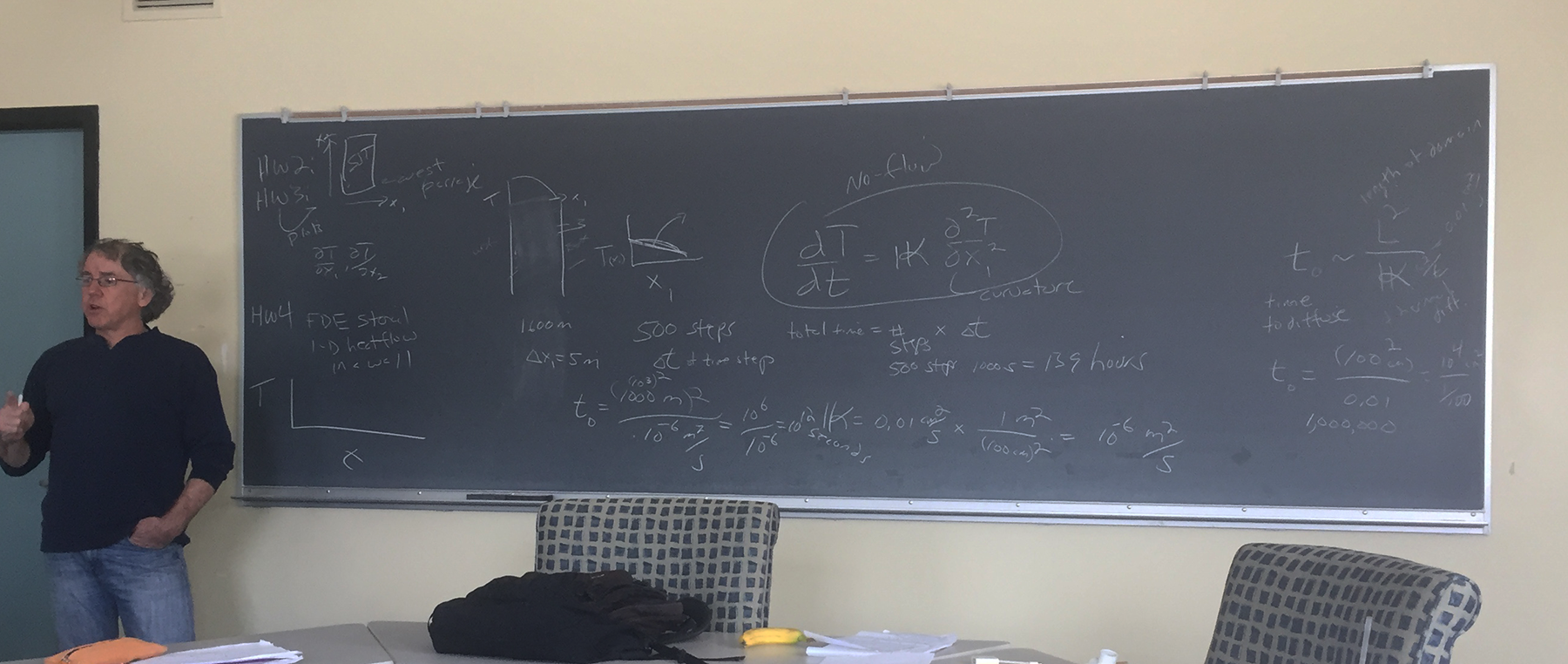
Chris mentioned the usefulness of the approximation as being applicable to thinking about cooking time for a Thanksgiving turkey (where the L is the radius of the approximate sphere of the turkey).
The take-home message of estimating equilibrium time so far, is that molecular heat diffusion is very slow. Chris suggested the next step was to look at the effect of eddies (kappaeddy — which has a good approximation of .15 meters2/second)
Chris suggested a next good step in our learning would be to consider the relationship between a Lagrangian perspective and a Eulerian one.
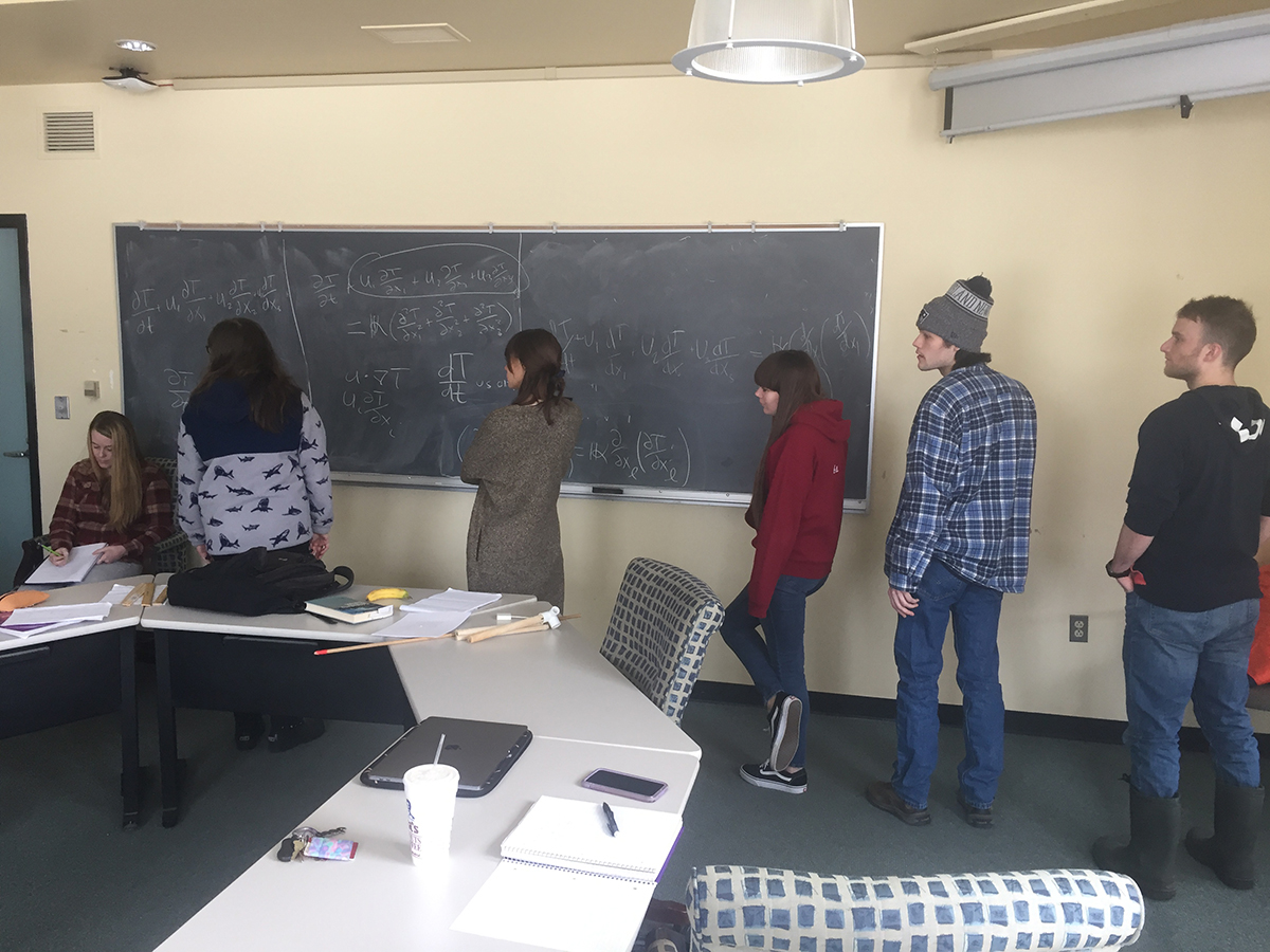
Chris had the students surround a parcel (with other parcels) and move around the room as a Lagrangian perspetive. Such is the perspective of speed using a speedometer in a car. We should use use a fat d vertical stroke to represent the Lagrangian perspective in a derivative.
On the other hand, the Eulerian perspective would be a speed gun that points to a certain volume of space to consider speed. We use a curly d stroke to represent the Eulerian perspective in a derivative.
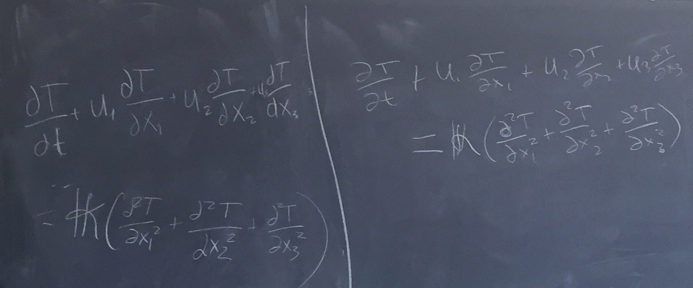
Chris reviewed a formula that relates the Lagrangian to the Eulerian:
dT/dt Lagrangian = dT/dt Eulerian + u . ▽T
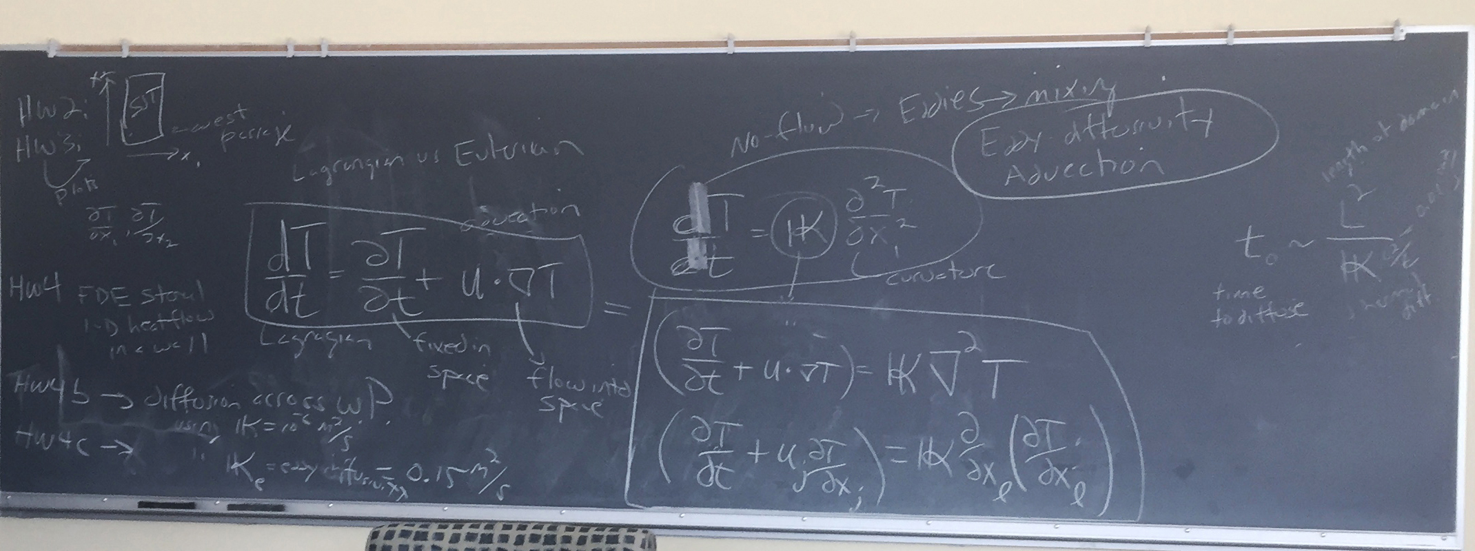
Students then performed a team challenge to expand the equation into its terms, with a reinforcing discussion between attempts:
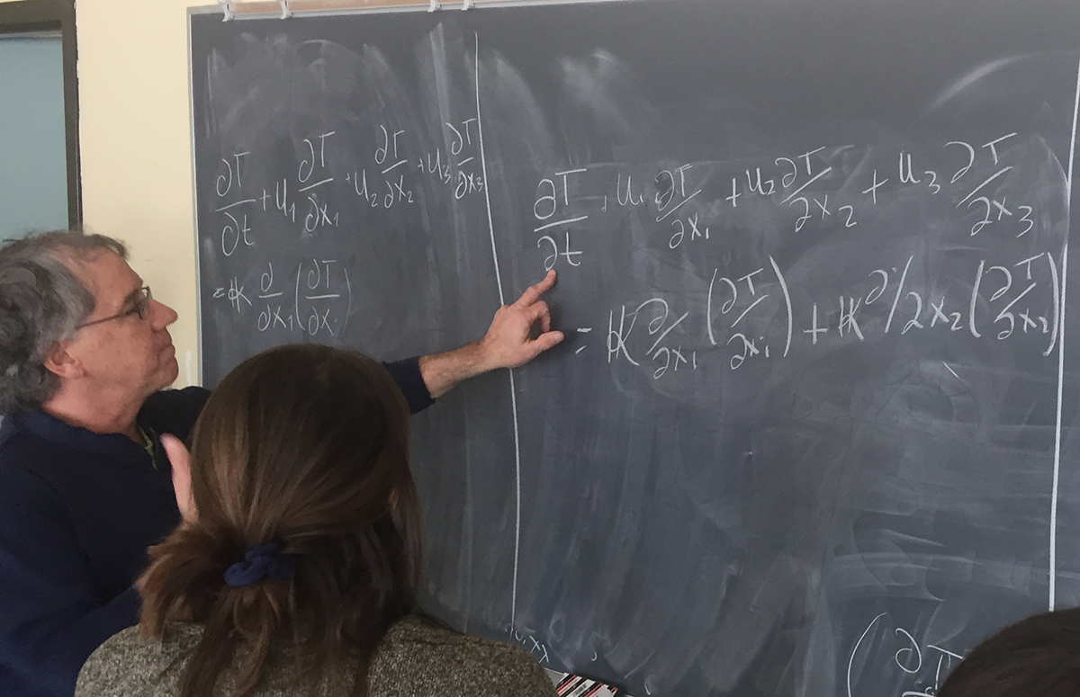
It took the teams four attempts to get the terms down in a minute (all but one team was then able to do so in time):
The students then simulated a Eulerian study of parcels moving through a fixed location (looking at slope changes and speed) by having a recorder sit in a chair and students pass by at different heights (height representing temperature at that time at the fixed position).
After redoing with different scenarios, students could visualize the change of temperature being affected by two things in unison: the speed by which the students passed and the difference between their heights as they did so. Temperature change could be the same when there were small changes passing by very fast or large changes passing by very slowly.
Chris then provided a series of heat flow scenarios to the student teams. Each team was to describe the magnitude of the variables listed at the bottom of each scenario:
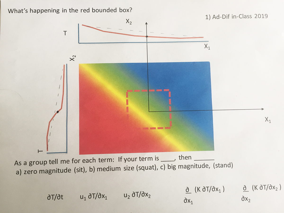
Students were asked to attempt describing the magnitude of variables in a handout scenario that included a diagonal flow for next class.
HW2 - Vectors in 2D water space
HW3 - Plots of vectors in 2D water space
HW4 - FDE equation and 1D heat flow node model (with fixed boundary nodes)
Chris asked students to calculate the time to reach equilibrium for homework #4a:
Sky got a value of 139 hours to reach equilibrium (using the equation on the blackboard - see below)
Chris reminded of the useful approximation formula for reaching t0 equilibrium:
t0 = L2/kappa
where L is the length of the heat diffusion space.
When applied to homework #4b:
t0 = 100 cm2/.02 = 1,000,000 seconds (or approximately 1000 years)
Using the long-hand equation we got 500,000 seconds (so not a bad first approximation to get a sense of magnitude)
Chris mentioned the usefulness of the approximation as being applicable to thinking about cooking time for a Thanksgiving turkey (where the L is the radius of the approximate sphere of the turkey).
The take-home message of estimating equilibrium time so far, is that molecular heat diffusion is very slow. Chris suggested the next step was to look at the effect of eddies (kappaeddy — which has a good approximation of .15 meters2/second)
Chris suggested a next good step in our learning would be to consider the relationship between a Lagrangian perspective and a Eulerian one.
Chris had the students surround a parcel (with other parcels) and move around the room as a Lagrangian perspetive. Such is the perspective of speed using a speedometer in a car. We should use use a fat d vertical stroke to represent the Lagrangian perspective in a derivative.
On the other hand, the Eulerian perspective would be a speed gun that points to a certain volume of space to consider speed. We use a curly d stroke to represent the Eulerian perspective in a derivative.
Chris reviewed a formula that relates the Lagrangian to the Eulerian:
dT/dt Lagrangian = dT/dt Eulerian + u . ▽T
Students then performed a team challenge to expand the equation into its terms, with a reinforcing discussion between attempts:
It took the teams four attempts to get the terms down in a minute (all but one team was then able to do so in time):
The students then simulated a Eulerian study of parcels moving through a fixed location (looking at slope changes and speed) by having a recorder sit in a chair and students pass by at different heights (height representing temperature at that time at the fixed position).
After redoing with different scenarios, students could visualize the change of temperature being affected by two things in unison: the speed by which the students passed and the difference between their heights as they did so. Temperature change could be the same when there were small changes passing by very fast or large changes passing by very slowly.
Chris then provided a series of heat flow scenarios to the student teams. Each team was to describe the magnitude of the variables listed at the bottom of each scenario:
Students were asked to attempt describing the magnitude of variables in a handout scenario that included a diagonal flow for next class.