

Class on November 27, 2018
We wrapped up module 2 in class with report presentations from student groups. Students worked with Narragansett Bay data and tried to develop NPZ models that would
provide results that aligned with the data. Students derived formulas that manipulated suggested models from the Miller reading, using inputs for precipitation, wind,
daylight, and irradiance. Formal presentations provided insights into different approaches and varying outputs in presented plots. One group described their fortuitous
adaptions particularly well (including the use of a maximium nutrient uptake parameter of 6 to spread out the phase space of component cycles). An annotated explanation
of the season affects seen in the observed data helped us comprehend the motivation of some techniques.
After a question and answer session with everyone in the room, Jeremy presented as if he were presenting as part of a project group. His clean and effective presentation style gave us much to ponder. He presented plots of formula parameters during the model run that very effectively showed their range over time. He discussed his formula adjustments for precipitation, wind, daylight, and irradiance. He showed the results of his most recent iteration and suggested four areas for improvement based on what the current iteration provided:
1. Add a delay of approximately 2 months for newly introduced nutrients to go through an ammonium to nitrate conversion, before being uptaken by phytoplankton.
2. Develop a detritus pool where nutrients that can be recycled sit as part of their cycle (initial attempts filled the model with what seemed like too much detritus.
3. Spend time in creating variables and formula that better reflect a realistic accounting of sources and sinks in the Narragansett Bay system.
4. Attune better to the impact of initial conditions for such sources and sinks as far as starting nutrients, phytoplankton, and zooplankton are involved.
Bruce then presented on his work investigating model parameters with a genetic programming approach. The code shared in class and through a case study tutorial below is just the beginning of an iterative process that should help gain insight into potentially improving a model fit to the observed data by tweaking parameters on a thoughtful model.
Genetic programming to investigate model parameters
(to follow along grab the NPZ_genetic_program-ode.ipynb notebook code from Sakai)
Anaconda provides many different artificial intelligence (AI), or machine learning, packages for use with a Python notebook. One popular one demonstrated in class is the deap Python package which can be installed into our Anaconda environments via the Terminal or Anaconca Command Prompt:
conda install -c conda-forge deap
The deap documentation then documents many methods for simulating an evolutionary process in a genetic program (GP).
The Wikipedia page on genetic programming suggests:
Step 1: Wrap the computational method with the genetic programming environment:
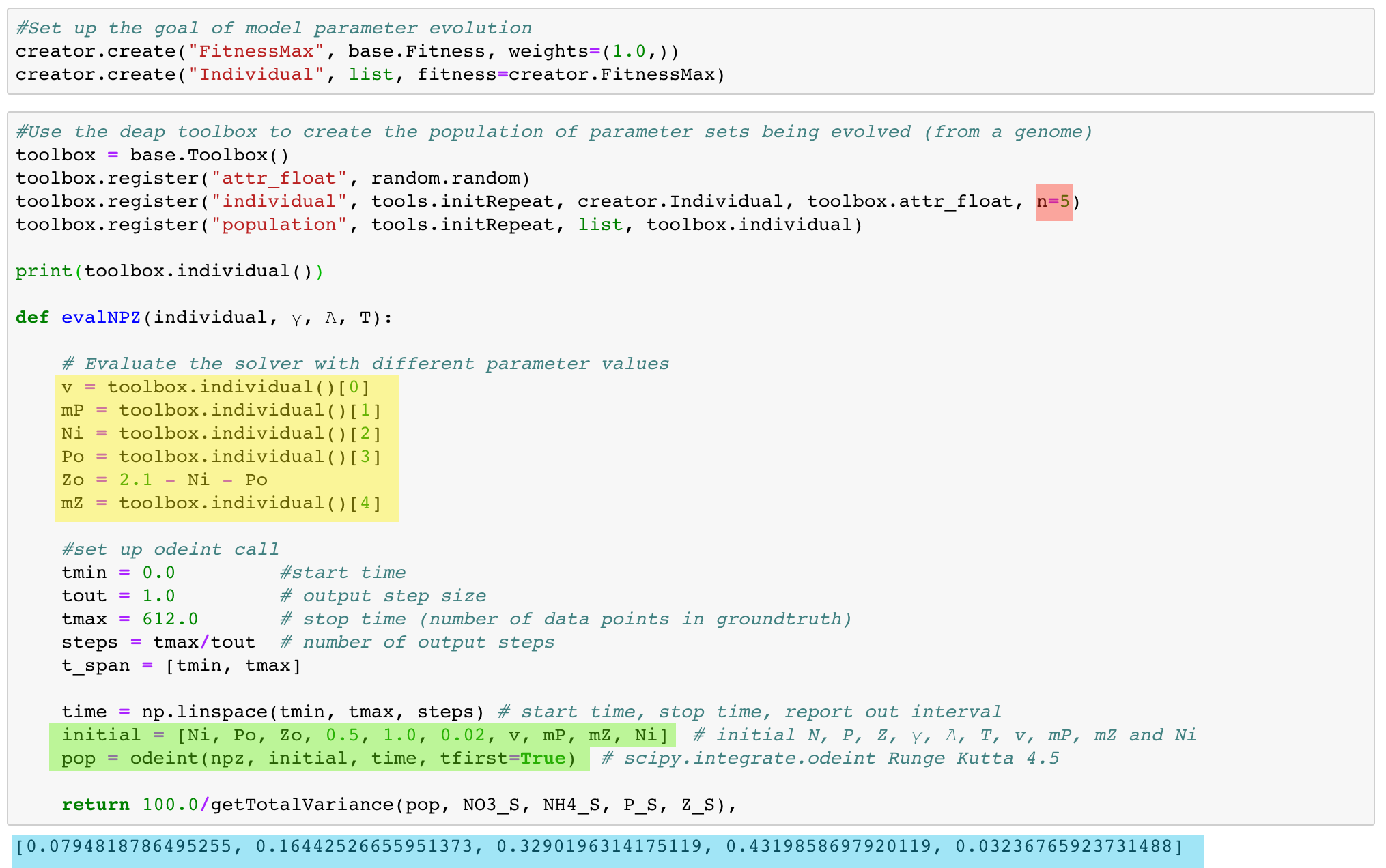
The code highlighted in green should look familiar as it initiates an ODE solver to solve for the NPZD model's differential equations. But instead of hardcoding parameter values in the model (the npz referenced as the first parameter to the odeint function call), one can pass them in as values being managed by the genetic program. For this example, we are passing in Ni, Po, Zo, γ, λ T, v, mP, mZ, and Ni as parameters. γ, λ and T are being held constant at 0.5, 1.0, and 0.02 for all model runs but they too could be managed by the genetic program if an analyst wanted to explore their potential effect as a range of values.
The code highlighted in yellow initializes the parameters based on the state of a genome that mimics how chromosomes retain and express information. As seen in the first six lines of code, the genetic program is created to evolve a maximum fitness process (to be described in detail later) on a population of digital chromosomes registered as an individuals comprising of five random floating point numbers (see the code highlighted in red). Those five floats are used to seed the parameter values highlighted in yellow.
Note that the code prints out an example of how individuals are generated from the genetic programming toolbox (using print(toolbox.individual()). The output of the print statement is highlighted in blue. For that individual chromosome, v would be set to 0.079..., Mp would be set to 0.164..., Ni would be set to 0.329..., Po would be set to 0.432..., and mZ would be set to 0.032... Zo is derived from Ni and Po.
So, there is a lot to do for Step 1, but it is mostly rote coding. The most important design step is in determining which parameters to explore within a digital chromosome.
Step 2: Create an evaluation function the genetic program can use to evolve better results:
Such a function is based on fitness and can be expressed in many ways with genetic programming tools. The usual caveat of be careful for what you wish for is prudent as the genetic program will pursue fitness at every step of its process. The evaluation function usually requires deep thought and often iterates upon the analyzing the results of using previous functions. In this case study, we use the following evaluation function:
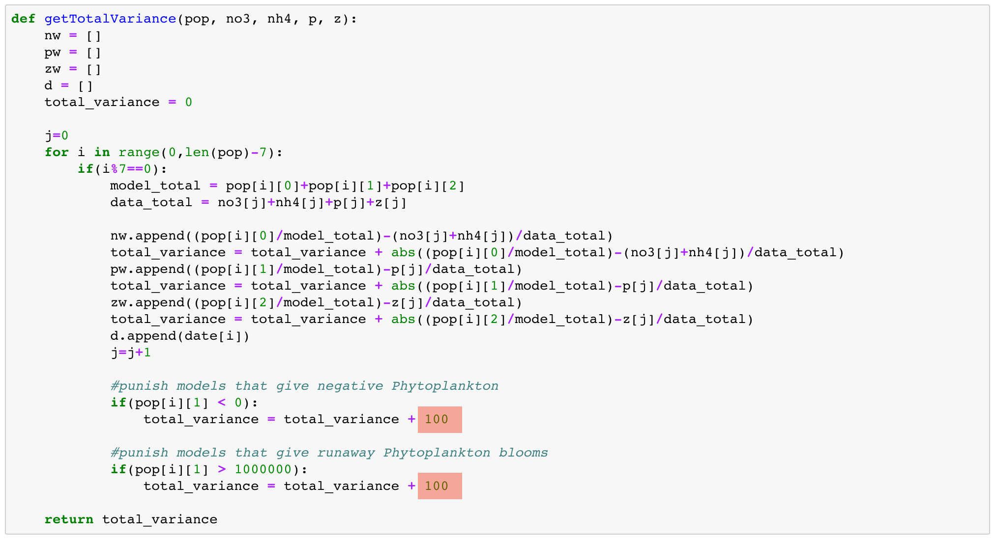
Since the data from Narragansett Bay is of a weekly resolution, we perform an analysis of every seventh day in the model output. The if statement that asks for data only where i%7==0 starts with day 0, and then day 7, day 14, day 21, etc. Wherever the day number divided by seven yields a remainder of exactly 0 (the % operator is called modulus).
The comparison of data v. model is done on the percentages of N, P, and Z in the total of the three at each timestep. The total_variance variable sums up the variance of the actual data versus model results data for N, P, and Z for each weekly time step. As seen in the red, we punish model results that provide extreme phytoplankton values at any timestep.
Again, many other evaluation functions can be inserted here instead. The analyst explores and continues to consider designs that will improve the results of the genetic program.
Refer again to the first code image. The last line of code in the evalNPZ function:
return 100.0/getTotalVariance(pop, NO3_S, NH4_S, P_S, Z_S)
converts the evaluation function into a value that can then be maximized by the genetic program (dividing the variance into 100 to provide values in a range from 0 to 2 - we could divide into any value to turn a minimizing fitness result into a maximizing fitness result.
In many cases, the brilliance of a human being makes an artificial intelligence process useful for doing meaningful work. It can be very difficult to come up with the fitness objective for any AI program (and genetic programming is but one approach of an increasing number of AI tools and approaches).
Step 3: Set up the genetic program to run as intended
There are many decisions to be made in setting up the genetic program. The code below is just one case study in terms of what is possible. The deap package provides documentation for the many tools that can be used. Basically, we are simulating a very basic evolutionary process by setting up a genetic program. We import the basic tool suite from deap using a familiar process:
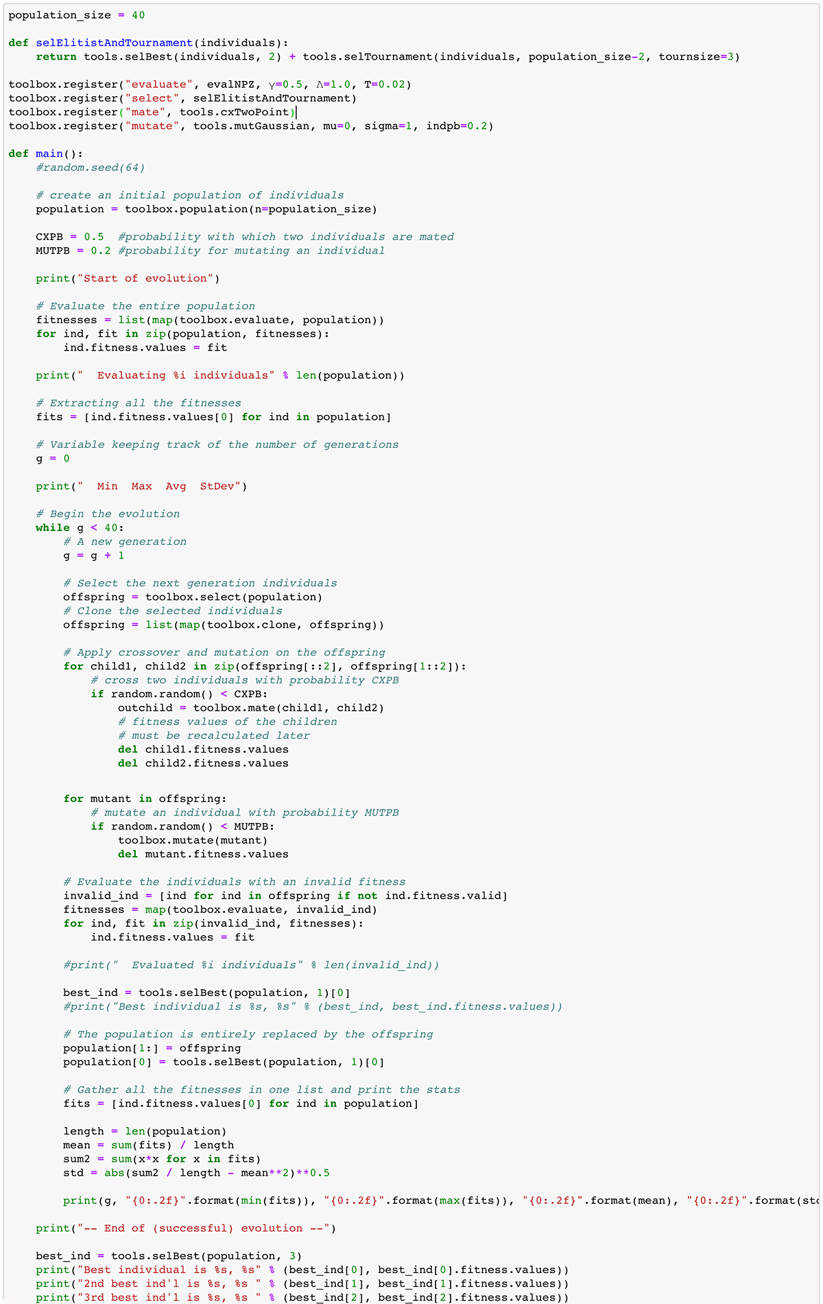
The number of generations increases the computation time and so there is often an end condition included in the code (for example, once reaching a desired minimal fitness). The number of individuals in the population increases computation time as does increasing the mating and mutation probabilities. The genetic program uses lots of random numbers performing its process. To reproduce the use of the same random numbers to perform the same run multiple times, we can use a seed integer (as seen in the line of code commented out: random.seed(64). Note also that many decisions are made in determining how to report upon the results of the program run.
Step 3 can take a lot of time to perform for those not familiar with a genetic program.
Step 4: Debug, Run, and Design further:
Debugging, running and redesigning based on run results can take a long time. In fact, this case study is nowhere near completion since the results are not all that interesting... yet. Debugging requires the same skills we can acquire from working with the Python language in a notebook environment. We use a lot of print functions to verify our assumptions or determine where something is going awry.
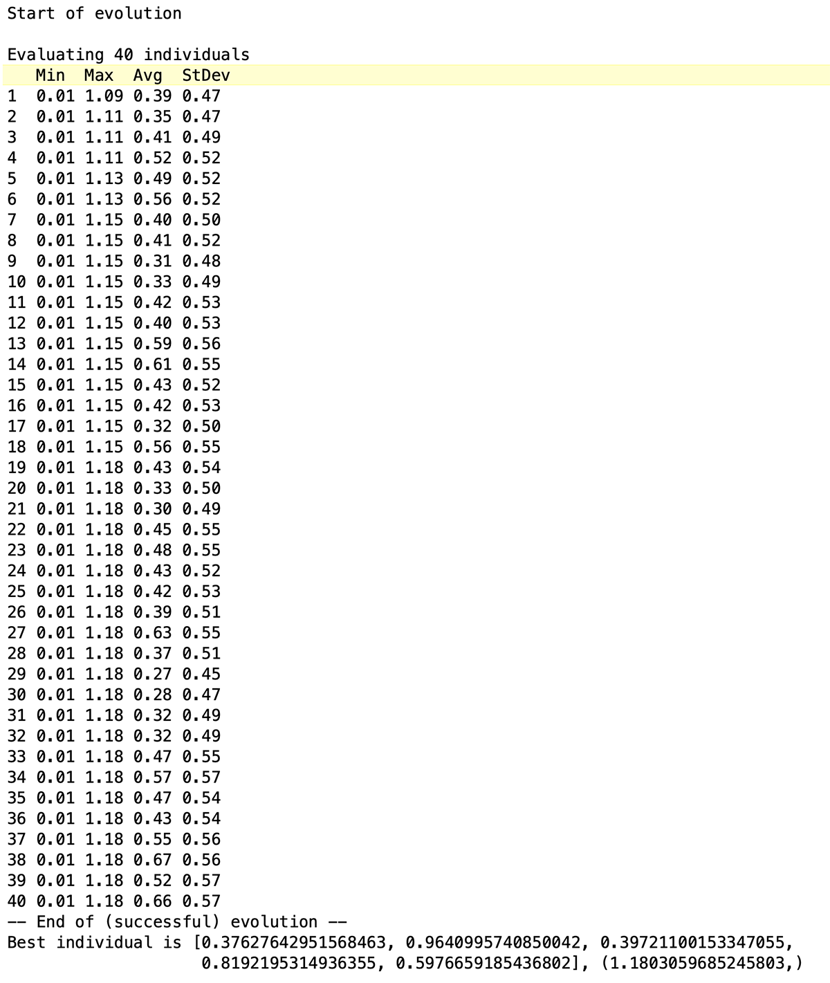
We run the genetic program by calling the function main() (since that's what we set the genetic program up in). Without a fixed random seed value, the run will be slightly different each time. One example of a run, using the code from above, appears below. Note that we coded to see the minimum individual chromosome fitness (still useful to retain digital recessive genes — or denes as described by genetic programming tutorials. We coded to track the maximum fitness (which we can confirm did increase for each generation in the run). We coded to see the average fitness (the most useful indicator in many situations), and the standard deviation (since we care about genetic diversity — coding in inbreeding or too much elitism limits the exploration of the parameter space).
We can code to see as many of the best resulting digital chromosomes in the final population (or, if not retaining them through elitism, we can create a hall of fame process that retains the best out of all the generations) as we want. Only one appears below, the best with its over 1.18 fitness evaluation. That digital chromosome suggests that setting the parameters to:
After a question and answer session with everyone in the room, Jeremy presented as if he were presenting as part of a project group. His clean and effective presentation style gave us much to ponder. He presented plots of formula parameters during the model run that very effectively showed their range over time. He discussed his formula adjustments for precipitation, wind, daylight, and irradiance. He showed the results of his most recent iteration and suggested four areas for improvement based on what the current iteration provided:
1. Add a delay of approximately 2 months for newly introduced nutrients to go through an ammonium to nitrate conversion, before being uptaken by phytoplankton.
2. Develop a detritus pool where nutrients that can be recycled sit as part of their cycle (initial attempts filled the model with what seemed like too much detritus.
3. Spend time in creating variables and formula that better reflect a realistic accounting of sources and sinks in the Narragansett Bay system.
4. Attune better to the impact of initial conditions for such sources and sinks as far as starting nutrients, phytoplankton, and zooplankton are involved.
Bruce then presented on his work investigating model parameters with a genetic programming approach. The code shared in class and through a case study tutorial below is just the beginning of an iterative process that should help gain insight into potentially improving a model fit to the observed data by tweaking parameters on a thoughtful model.
Genetic programming to investigate model parameters
(to follow along grab the NPZ_genetic_program-ode.ipynb notebook code from Sakai)
Anaconda provides many different artificial intelligence (AI), or machine learning, packages for use with a Python notebook. One popular one demonstrated in class is the deap Python package which can be installed into our Anaconda environments via the Terminal or Anaconca Command Prompt:
conda install -c conda-forge deap
The deap documentation then documents many methods for simulating an evolutionary process in a genetic program (GP).
The Wikipedia page on genetic programming suggests:
In artificial intelligence, genetic programming (GP) is a technique whereby computer programs are encoded as a set of genes that are then modified (evolved) using an evolutionary algorithm (often a genetic algorithm, "GA") — it is an application of (for example) genetic algorithms where the space of solutions consists of computer programs. The results are computer programs that are able to perform well in a predefined task. The methods used to encode a computer program in an artificial chromosome and to evaluate its fitness with respect to the predefined task are central in the GP technique and still the subject of active research.What follows is a case study in using genetic programming to perform an analysis on a complex system. The steps can be generalized for use with many other GP tools and subjects of analysis:
Step 1: Wrap the computational method with the genetic programming environment:
toolbox.register("evaluate", evalNPZ, γ=0.5,λ=1.0, T=0.02)
toolbox.register("select", selElitistAndTournament, k_tournament=population_size-3, tournsize=3)
toolbox.register("mate", tools.cxTwoPoint)
toolbox.register("mutate", tools.mutGaussian, mu=0, sigma=1, indpb=0.2)
The function evalNPZ performs the model computation within the context of the genetic programming environment:
The code highlighted in green should look familiar as it initiates an ODE solver to solve for the NPZD model's differential equations. But instead of hardcoding parameter values in the model (the npz referenced as the first parameter to the odeint function call), one can pass them in as values being managed by the genetic program. For this example, we are passing in Ni, Po, Zo, γ, λ T, v, mP, mZ, and Ni as parameters. γ, λ and T are being held constant at 0.5, 1.0, and 0.02 for all model runs but they too could be managed by the genetic program if an analyst wanted to explore their potential effect as a range of values.
The code highlighted in yellow initializes the parameters based on the state of a genome that mimics how chromosomes retain and express information. As seen in the first six lines of code, the genetic program is created to evolve a maximum fitness process (to be described in detail later) on a population of digital chromosomes registered as an individuals comprising of five random floating point numbers (see the code highlighted in red). Those five floats are used to seed the parameter values highlighted in yellow.
Note that the code prints out an example of how individuals are generated from the genetic programming toolbox (using print(toolbox.individual()). The output of the print statement is highlighted in blue. For that individual chromosome, v would be set to 0.079..., Mp would be set to 0.164..., Ni would be set to 0.329..., Po would be set to 0.432..., and mZ would be set to 0.032... Zo is derived from Ni and Po.
So, there is a lot to do for Step 1, but it is mostly rote coding. The most important design step is in determining which parameters to explore within a digital chromosome.
Step 2: Create an evaluation function the genetic program can use to evolve better results:
Such a function is based on fitness and can be expressed in many ways with genetic programming tools. The usual caveat of be careful for what you wish for is prudent as the genetic program will pursue fitness at every step of its process. The evaluation function usually requires deep thought and often iterates upon the analyzing the results of using previous functions. In this case study, we use the following evaluation function:
Since the data from Narragansett Bay is of a weekly resolution, we perform an analysis of every seventh day in the model output. The if statement that asks for data only where i%7==0 starts with day 0, and then day 7, day 14, day 21, etc. Wherever the day number divided by seven yields a remainder of exactly 0 (the % operator is called modulus).
The comparison of data v. model is done on the percentages of N, P, and Z in the total of the three at each timestep. The total_variance variable sums up the variance of the actual data versus model results data for N, P, and Z for each weekly time step. As seen in the red, we punish model results that provide extreme phytoplankton values at any timestep.
Again, many other evaluation functions can be inserted here instead. The analyst explores and continues to consider designs that will improve the results of the genetic program.
Refer again to the first code image. The last line of code in the evalNPZ function:
return 100.0/getTotalVariance(pop, NO3_S, NH4_S, P_S, Z_S)
converts the evaluation function into a value that can then be maximized by the genetic program (dividing the variance into 100 to provide values in a range from 0 to 2 - we could divide into any value to turn a minimizing fitness result into a maximizing fitness result.
In many cases, the brilliance of a human being makes an artificial intelligence process useful for doing meaningful work. It can be very difficult to come up with the fitness objective for any AI program (and genetic programming is but one approach of an increasing number of AI tools and approaches).
Step 3: Set up the genetic program to run as intended
There are many decisions to be made in setting up the genetic program. The code below is just one case study in terms of what is possible. The deap package provides documentation for the many tools that can be used. Basically, we are simulating a very basic evolutionary process by setting up a genetic program. We import the basic tool suite from deap using a familiar process:
from deap import algorithms
from deap import base
from deap import creator
from deap import tools
from deap import gp
and they are then available to our genetic program in the Python notebook. Some significant choices made in setting up the code include:
- The number of generations to run the program for (40 in the code below, as seen by the line while g < 40)
- The size of the population (number of chromosome individuals) to evolve (40 as seen by the first line in the code below)
- The evaluation criteria (described in Step 1 above) as our evalNPZ function with three fixed parameters
- The selection method for selecting which individuals continue on to a successive generation
- The mating method for mating two individuals to create two offspring (based on a CXPB variable for probability of mating)
- The mutation method for mutating a chromosome (usually a much higher rate that what would occur in nature - probability based on the MUTPB variable set to 20%)
The number of generations increases the computation time and so there is often an end condition included in the code (for example, once reaching a desired minimal fitness). The number of individuals in the population increases computation time as does increasing the mating and mutation probabilities. The genetic program uses lots of random numbers performing its process. To reproduce the use of the same random numbers to perform the same run multiple times, we can use a seed integer (as seen in the line of code commented out: random.seed(64). Note also that many decisions are made in determining how to report upon the results of the program run.
Step 3 can take a lot of time to perform for those not familiar with a genetic program.
Step 4: Debug, Run, and Design further:
Debugging, running and redesigning based on run results can take a long time. In fact, this case study is nowhere near completion since the results are not all that interesting... yet. Debugging requires the same skills we can acquire from working with the Python language in a notebook environment. We use a lot of print functions to verify our assumptions or determine where something is going awry.
We run the genetic program by calling the function main() (since that's what we set the genetic program up in). Without a fixed random seed value, the run will be slightly different each time. One example of a run, using the code from above, appears below. Note that we coded to see the minimum individual chromosome fitness (still useful to retain digital recessive genes — or denes as described by genetic programming tutorials. We coded to track the maximum fitness (which we can confirm did increase for each generation in the run). We coded to see the average fitness (the most useful indicator in many situations), and the standard deviation (since we care about genetic diversity — coding in inbreeding or too much elitism limits the exploration of the parameter space).
We can code to see as many of the best resulting digital chromosomes in the final population (or, if not retaining them through elitism, we can create a hall of fame process that retains the best out of all the generations) as we want. Only one appears below, the best with its over 1.18 fitness evaluation. That digital chromosome suggests that setting the parameters to:
v  = 0.37627642951568463,
mP = 0.9640995740850042,
Ni = 0.39721100153347055,
Po = 0.8192195314936355,
mZ = 0.5976659185436802
provided the lowest total variance of all the combinations of parameters tried in forty generations of forty individuals each.